REVIEW 1 major objections 5 minor 2 cited by
Hypocoercivity properties of adaptive Langevin dynamics
T0 review · 1 major / 5 minor · reviewed 2026-08-14 · deepseek-v4-flash
Pith's one-line read Adaptive Langevin sampling converges exponentially fast to its target measure.
desk verdict Solid hypocoercivity proof for Adaptive Langevin with an honest parameter-dependent rate; the main gap is the idealized state-independent noise model that limits how far the theorem reaches into stochastic-gradient MCMC. read the letter →
The pith
A machine-rendered reading of the paper's core claim, the machinery that carries it, and where it could break.
The reading
What carries the argument
The argument is carried by a modified norm $\mathcal{H}(\phi)=\tfrac12\|\phi\|^2_{L^2(\pi)}+a_{\varepsilon,\gamma}\langle A_\varepsilon\phi,\phi\rangle_{L^2(\pi)}$, where $A_\varepsilon$ is a regularizing operator constructed from the antisymmetric part of the generator, that is, the Hamiltonian part plus the scaled feedback-control part. The definition of $A_\varepsilon$ switches at $\varepsilon=1$: for $\varepsilon\le 1$ it regularizes the Hamiltonian transport, while for $\varepsilon>1$ the generator is first multiplied by $\varepsilon$ and the feedback part is regularized instead. This switch is what makes the partial coercivity estimate hold with the correct $\varepsilon$-dependent rate. The resulting coercivity of $-L_{\mathrm{AdL}}$ in the modified scalar product gives the exponential decay via a differential-inequality argument, and the same coercivity bounds the inverse generator, which is the input to the central limit theorem.
What would settle it
On the quadratic potential $U(q)=q^2/2$, compute the spectral gap of a finite spectral discretization of $-L_{\mathrm{AdL}}$ along a curve with $\gamma\varepsilon^2$ fixed and $\varepsilon\to0$; Theorem 2.1 requires the gap to stay at least a fixed fraction of $\gamma\varepsilon^2$, so a gap decaying faster than that bound would falsify the rate. Separately, replacing the additive gradient noise in a simulation by state-dependent noise of the same mean and comparing the empirical stationary distribution with $e^{-\beta U}$ would test whether the invariant-measure assumption carries over.
Extended reading notes
Core claim
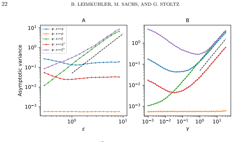
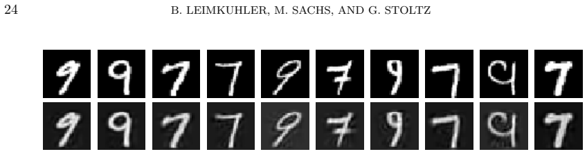
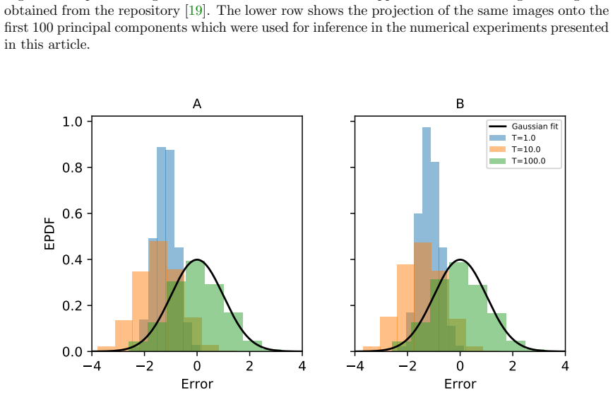
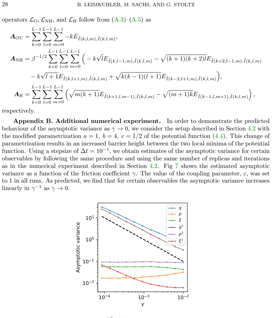
The central claim is Theorem 2.1: for any $\varepsilon,\gamma>0$, the semigroup $e^{tL_{\mathrm{AdL}}}$ contracts in $L^2(\pi)$ toward $\int\phi\,d\pi$ with rate at least $\lambda\min(\gamma,\gamma^{-1},\gamma\varepsilon^2,(\gamma\varepsilon^2)^{-1})$. The proof exhibits a modified norm in which the generator is coercive, and then applies a differential-inequality estimate. The invertibility of the generator on mean-zero functions follows, and with it a functional central limit theorem: $\sqrt{t}(\hat\phi_t-\mathbb{E}_\pi\phi)$ converges to a centered normal distribution with variance $2\langle -L_{\mathrm{AdL}}^{-1}\Pi_0\phi,\Pi_0\phi\rangle_{L^2(\pi)}$, bounded above by $O(\max(\gamma,\gamma^{-1},\gamma\varepsilon^2,(\gamma\varepsilon^2)^{-1}))$. In the large-thermostat-mass limit $\varepsilon\to\infty$, the asymptotic variance approaches the underdamped Langevin variance at order $1/\varepsilon$, so the added thermostat does not degrade efficiency in that regime. Numerical experiments on a double-well model and on Bayesian logistic regression for handwritten-digit classification confirm the predicted scalings and the normal limit law.
Load-bearing premise
The load-bearing premise is that gradient corruption is an additive white-noise term with constant covariance matrix $\sigma_G^2 I$, independent of position; the invariant measure and the whole generator decomposition are built on that form, and real minibatch gradient noise only approximates it.
Editorial extensions
If this is right
- Users of ALD can estimate posterior expectations from one long trajectory and attach asymptotically valid normal error bars, provided the gradient noise is approximately additive and white.
- The rate formula identifies the dangerous regimes: mixing degrades as $\gamma\to0$ or $\gamma\to\infty$, and as $\nu=\varepsilon^2\to\infty$ or $\nu\to0$, with the precise power law $\min(\gamma,\gamma^{-1},\gamma\varepsilon^2,(\gamma\varepsilon^2)^{-1})$.
- The inverse-generator bound of order $\max(\gamma,\gamma^{-1},\gamma\varepsilon^2,(\gamma\varepsilon^2)^{-1})$ tells practitioners how long to integrate: of order that maximum will bring the variance of a time average to order one.
- As $\varepsilon\to\infty$, ALD inherits the sampling efficiency of underdamped Langevin dynamics, since the asymptotic variance converges to the Langevin value at rate $1/\varepsilon$.
Reading between the lines
- In the actual minibatch setting the gradient residual is state-dependent and only approximately normal, so the theorem does not by itself certify the Bayesian posterior; a natural test would be to measure the bias introduced by a state-dependent $\sigma_G^2(q)$ and compare with the white-noise idealization.
- The $\varepsilon\to0$ singular limit, where the feedback dynamics dominates on level sets of $\Phi=\xi^2+|p|^2-(2n/\beta)\ln|p|^2$, suggests a homogenized slow description that could yield sharp asymptotic variance predictions; the paper does not carry this out.
- The same modified-norm machinery should transfer to other thermostatted sampling schemes whose generator splits into symmetric and antisymmetric parts, giving explicit rates in terms of their parameters.
- A quantitative check of the theorem's boundary: increasing minibatch size lowers gradient-noise variance; the theory predicts the rate improves as $\gamma$ decreases toward order one, which is testable on a fixed data set.
Signed reviews
Editorial analysis
A structured set of objections, weighed in public.
Referee Report
Summary. The paper analyzes the Adaptive Langevin dynamics SDE, a sous-thermostatted Langevin system with an additional gradient-noise term of unknown, constant intensity. After rescaling the thermostat variable, the authors decompose the generator and prove (Theorem 2.1) exponential convergence in L^2(pi) for the semigroup, with a rate lower bound proportional to min(gamma, 1/gamma, gamma epsilon^2, 1/(gamma epsilon^2)). They then infer invertibility of the generator on the mean-zero subspace and derive a central limit theorem for ergodic averages with bounds on the asymptotic variance. A companion result (Proposition 3.1) shows that, for observables depending only on (q,p), the asymptotic variance converges to that of standard underdamped Langevin dynamics as epsilon -> infinity. The theoretical scaling is tested numerically by Galerkin computation of the spectral gap, by simulation of asymptotic variances, and by a Bayesian logistic-regression example on MNIST using a minibatch gradient estimator.
Significance. If the results are correct, this is a substantial contribution: it gives the first quantitative hypocoercivity estimate for Adaptive Langevin dynamics with explicit dependence on the friction and thermostat-mass parameters, and it upgrades earlier qualitative results (e.g., Herzog's Lyapunov-function analysis) to an L^2 rate and a CLT. The proof is self-contained and analytic, with no fitted parameters; the derived scaling is concrete and falsifiable, and the Galerkin numerics in Section 4.1 support the predicted exponents. The Bayesian-sampling application illustrates the intended use, although the bridge from the idealized model to the minibatch setting requires a modeling assumption that is not exactly satisfied.
major comments (1)
- [Section 2.4, Proposition 2.2 and equation (2.13)] The statement of Proposition 2.2 fixes the regularization parameter as a_{\varepsilon,\gamma} = a \min(\gamma, \gamma^{-1}, \gamma\varepsilon^2, (\gamma\varepsilon^2)^{-1}), but the proof in the paragraph "For \varepsilon > 1" instead chooses a_{\varepsilon,\gamma} = a \min(\gamma\varepsilon, (\gamma\varepsilon)^{-1}). These two choices differ by a factor \varepsilon in the regime \varepsilon > 1: for \gamma\varepsilon < 1 the stated formula gives a\gamma while the proof uses a\gamma\varepsilon, and for \gamma\varepsilon > 1 it gives a/(\gamma\varepsilon^2) while the proof uses a/(\gamma\varepsilon). With the stated formula, the determinant condition (2.24) yields a lower bound of order \gamma/\varepsilon (respectively 1/(\gamma\varepsilon^3)) instead of \gamma (respectively 1/(\gamma\varepsilon^2)) in these regimes, so the uniform constant \tilde{\lambda} in Proposition 2.2 cannot exist. The proposition statement must be corrected, for example by giving the piecewise definition of a_{\varepsilon,\gamma} that is actually used in the proof, so that the statement and proof are consistent.
minor comments (5)
- [Appendix C.2, ODABADO algorithm] In the last momentum update of the ODABADO algorithm, the text reads p_{k+1} = \alpha(\zeta_{k+1}, \Delta t/2) p_k + G(\sigma_A, \zeta_{k+1}, \Delta t/2) R_{k+1/2}; for consistency with the symmetric splitting (C.12), the argument should be \hat{p}_{k+1/2} (the value after the gradient-noise substep), not p_k.
- [Section 4.3 and Appendix C.2] The numerical CLT demonstration for Bayesian logistic regression uses a minibatch gradient estimator, whose residual noise is state-dependent and only approximately Gaussian, whereas the ODABADO integrator is derived under the assumption in Appendix C.2 that the residual is Gaussian and independent of q_k. The text should state explicitly in Section 4.3 that the experiment is an empirical check under this modeling assumption and is not a direct consequence of Corollary 2 for the actual subsampled process.
- [Section 3, Corollaries 1 and 2] The word "Collorary" appears in place of "Corollary" in the headings/callouts for Corollary 1 and Corollary 2; also "trajecotry" appears in Section 4.2 and "different" appears in Section 4.2.
- [Section 3 title] The section title "Pathwise ergodicity and functional central limit theorem" promises a functional CLT, but only the ordinary CLT is stated in Corollary 2; either add the functional CLT or change the title.
- [Equation (3.5)] In the solvability condition (3.5), the notation \Pi_0\phi is ambiguous: it should be made clear that the integral is a partial average over (q,p), which vanishes because \phi is restricted to functions of (q,p) only in Proposition 3.1; otherwise it can be mistaken for the global projection defined in (2.8).
Circularity Check
No circularity: the exponential convergence theorem is derived analytically from the generator decomposition and the external hypocoercivity framework, with numerical experiments testing the derived scalings.
full rationale
The paper's central claim (Theorem 2.1) is an analytically derived L2 hypocoercivity estimate for the adaptive Langevin SDE (2.4). The proof chain is self-contained: the generator is decomposed as L_AdL = L_H + gamma L_O + epsilon^{-1} L_NH; the invariant measure (1.3) is verified by direct adjoint computations; the modified norm H and regularization operator A_epsilon are constructed from that decomposition; Proposition 2.2 establishes coercivity, and Theorem 2.1 follows by a Grönwall argument. No parameter is fitted to data, and the rate lower bound (2.12) follows from the proof rather than being imposed. The numerical sections test the predicted scalings (e.g., the spectral gap in the Hermite Galerkin subspace and the CLT residuals) rather than tune parameters to force agreement. Citations to the authors' earlier work [16, 33, 22] introduce the dynamics and numerical integrators, but they do not carry the convergence proof; the key external inputs are the general hypocoercivity framework of Dolbeault–Mouhot–Schmeiser and the CLT criterion of Bhattacharya. The acknowledged assumption in Appendix C.2 that minibatch gradient noise is Gaussian and state-independent is a limitation on the application to subsampled Bayesian inference, not a circular step in the mathematical derivation.
Assumptions & free parameters
assumptions (4)
- domain assumption Assumption 1: U is smooth, pi_q satisfies a Poincare inequality, and Delta U <= c1 + (c2/2)|grad U|^2 with c2 in [0,1), |grad^2 U| <= c3(1+|grad U|).
- domain assumption Gradient perturbation is an additive Ito white-noise process sigma_G dW_G with constant sigma_G.
- standard math Technical boundedness estimates from [9, Section 3] for operators such as partial^2_{q_i,q_j}(1-P_q)(1+Pi grad*_q grad_q Pi)^-1.
- standard math Bhattacharya's functional central limit theorem [2] for ergodic Markov processes.
Cite this review
Pith. "Pith review of Hypocoercivity properties of adaptive Langevin dynamics." pith.science (2026). https://pith.science/paper/OEW3W7KB
@misc{pith2026190809363,
  author       = {Pith},
  title        = {Pith review of: Hypocoercivity properties of adaptive Langevin dynamics},
  year         = {2026},
  howpublished = {\url{https://pith.science/paper/OEW3W7KB}},
  note         = {Machine review of arXiv:1908.09363}
}
read the original abstract
Adaptive Langevin dynamics is a method for sampling the Boltzmann-Gibbs distribution at prescribed temperature in cases where the potential gradient is subject to stochastic perturbation of unknown magnitude. The method replaces the friction in underdamped Langevin dynamics with a dynamical variable, updated according to a negative feedback loop control law as in the Nos\'e-Hoover thermostat. Using a hypocoercivity analysis we show that the law of Adaptive Langevin dynamics converges exponentially rapidly to the stationary distribution, with a rate that can be quantified in terms of the key parameters of the dynamics. This allows us in particular to obtain a central limit theorem with respect to the time averages computed along a stochastic path. Our theoretical findings are illustrated by numerical simulations involving classification of the MNIST data set of handwritten digits using Bayesian logistic regression.
Figures


Figures from the paper (4 more)

Forward citations
Cited by 2 Pith papers
-
Hypocoercivity meets lifts
A unified hypocoercivity framework shows adaptive Langevin dynamics is a near-optimal lift, and proves the generalized Langevin equation cannot beat square-root speedup.
-
Partitioned integrators for thermodynamic parameterization of neural networks
Layer-partitioned Langevin integrators (LOL and AdLaLa) train single hidden layer perceptrons faster, more accurately, and more robustly than SGD/Adam on hard spiral and trigonometric classification problems.
Reference graph
Works this paper leans on
- [1]
-
[2]
R. N. Bhattacharya, On the functional central limit theorem and the law of the iterated logarithm for Markov processes, Zeitschrift f¨ ur Wahrscheinlichkeitstheorie und verwandte Gebiete, 60 (1982), pp. 185–201
work page 1982
-
[3]
N. Bou-Rabee and H. Owhadi , Long-run accuracy of variational integrators in the stochastic context , SIAM Journal on Numerical Analysis, 48 (2010), pp. 278–297
work page 2010
- [4]
-
[5]
T. Chen, E. Fox, and C. Guestrin, Stochastic gradient Hamiltonian Monte Carlo, in International Conference on Machine Learning, 2014, pp. 1683–1691
work page 2014
- [6]
-
[7]
N. Ding, Y. Fang, R. Babbush, C. Chen, R. D. Skeel, and H. Neven , Bayesian sampling using stochastic gradient thermostats, in Advances in neural information processing systems, 2014, pp. 3203–3211
work page 2014
-
[8]
J. Dolbeault, C. Mouhot, and C. Schmeiser , Hypocoercivity for kinetic equations with linear relaxation terms, C. R. Math. Acad. Sci. Paris, 347 (2009), pp. 511–516
work page 2009
Show all 37 references
-
[9]
Dolbeault, C
J. Dolbeault, C. Mouhot, and C. Schmeiser , Hypocoercivity for linear kinetic equations conserving mass , Transactions of the American Mathematical Society, 367 (2015), pp. 3807–3828
2015
-
[10]
Eberle, Reflection coupling and Wasserstein contractivity without convexity , Comptes Rendus Mathema- tique, 349 (2011), pp
A. Eberle, Reflection coupling and Wasserstein contractivity without convexity , Comptes Rendus Mathema- tique, 349 (2011), pp. 1101–1104
2011
-
[11]
Eberle, A
A. Eberle, A. Guillin, and R. Zimmer, Couplings and quantitative contraction rates for Langevin dynamics , Ann. Probab., 47 (2019), pp. 1982–2010
2019
-
[12]
Hairer and J
M. Hairer and J. C. Mattingly , Yet another look at Harris ergodic theorem for Markov chains , in Seminar on Stochastic Analysis, Random Fields and Applications VI, vol. 63, Springer, 2011, pp. 109–117
2011
-
[13]
D. P. Herzog, Exponential relaxation of the Nos´ e-Hoover equation under Brownian heating, Communications in Mathematical Sciences, 16 (2018), pp. 2231–2260
2018
-
[14]
H¨ormander, Hypoelliptic second order differential equations, Acta Math., 119 (1967), pp
L. H¨ormander, Hypoelliptic second order differential equations, Acta Math., 119 (1967), pp. 147–171
1967
-
[15]
Iacobucci, S
A. Iacobucci, S. Olla, and G. Stoltz , Convergence rates for nonequilibrium Langevin dynamics , Annales math´ ematiques du Qu´ ebec, 43 (2019), pp. 73–98
2019
-
[16]
Jones and B
A. Jones and B. Leimkuhler, Adaptive stochastic methods for sampling driven molecular systems, The Journal of Chemical Physics, 135 (2011), p. 084125
2011
-
[17]
Kliemann, Recurrence and invariant measures for degenerate diffusions, Ann
W. Kliemann, Recurrence and invariant measures for degenerate diffusions, Ann. Probab., 15 (1987), pp. 690– 707
1987
-
[18]
Kopec , Weak backward error analysis for Langevin process , BIT Numerical Mathematics, 55 (2015), pp
M. Kopec , Weak backward error analysis for Langevin process , BIT Numerical Mathematics, 55 (2015), pp. 1057–1103
2015
-
[19]
LeCun and C
Y. LeCun and C. Cortes , MNIST handwritten digit database , (2010), http://yann.lecun.com/exdb/mnist/
2010
-
[20]
Leimkuhler and C
B. Leimkuhler and C. Matthews, Molecular Dynamics: With Deterministic and Stochastic Numerical Meth- ods, Interdisciplinary Applied Mathematics, Springer, 2015
2015
-
[21]
Leimkuhler, C
B. Leimkuhler, C. Matthews, and G. Stoltz , The computation of averages from equilibrium and nonequi- librium Langevin molecular dynamics , IMA Journal of Numerical Analysis, 36 (2015), pp. 13–79
2015
-
[22]
Leimkuhler and X
B. Leimkuhler and X. Shang , Adaptive thermostats for noisy gradient systems , SIAM Journal on Scientific Computing, 38 (2016), pp. A712–A736
2016
-
[23]
Leli `evre and G
T. Leli `evre and G. Stoltz , Partial differential equations and stochastic methods in molecular dynamics , Acta Numerica, 25 (2016), pp. 681–880
2016
-
[24]
J. C. Mattingly, A. M. Stuart, and D. J. Higham, Ergodicity for SDEs and approximations: locally Lipschitz vector fields and degenerate noise , Stochastic Processes and their Applications, 101 (2002), pp. 185–232
2002
-
[25]
S. P. Meyn and R. L. Tweedie , Stability of Markovian processes II: Continuous-time processes and sampled chains, Advances in Applied Probability, 25 (1993), pp. 487–517
1993
-
[26]
S. P. Meyn and R. L. Tweedie , Markov Chains and Stochastic Stability , Springer Science & Business Media, HYPOCOERCIVITY PROPERTIES OF ADAPTIVE LANGEVIN DYNAMICS 27 2012
2012
-
[27]
Nos ´e, A unified formulation of the constant temperature molecular dynamics methods , The Journal of Chemical Physics, 81 (1984), pp
S. Nos ´e, A unified formulation of the constant temperature molecular dynamics methods , The Journal of Chemical Physics, 81 (1984), pp. 511–519
1984
-
[28]
G. A. Pavliotis, Stochastic Processes and Applications, Springer, 2016
2016
-
[29]
G. A. Pavliotis and A. Vogiannou, Diffusive transport in periodic potentials: underdamped dynamics , Fluc- tuation and Noise Letters, 08 (2008), pp. L155–L173
2008
-
[30]
Rey-Bellet, Ergodic properties of Markov processes, in Open Quantum Systems II, S
L. Rey-Bellet, Ergodic properties of Markov processes, in Open Quantum Systems II, S. Attal, A. Joye, and C.-A. Pillet, eds., vol. 1881 of Lecture Notes in Mathematics, Springer, 2006, pp. 1–39
2006
-
[31]
Roussel and G
J. Roussel and G. Stoltz , Spectral methods for Langevin dynamics and associated error estimates , ESAIM Math. Model. Numer. Anal., 52 (2018), pp. 1051–1083
2018
-
[32]
Sachs, B
M. Sachs, B. Leimkuhler, and V. Danos , Langevin dynamics with variable coefficients and nonconservative forces: From stationary states to numerical methods , Entropy, 19 (2017), p. 647
2017
-
[33]
Shang, Z
X. Shang, Z. Zhu, B. Leimkuhler, and A. J. Storkey , Covariance-controlled adaptive Langevin thermostat for large-scale Bayesian sampling, in Advances in Neural Information Processing Systems, 2015, pp. 37–45
2015
-
[34]
D. Talay, Stochastic Hamiltonian systems: exponential convergence to the invariant measure, and discretiza- tion by the implicit Euler scheme , Markov Processes and Related Fields, 8 (2002), pp. 163–198
2002
-
[35]
V´arnai, N
C. V´arnai, N. Bernstein, L. Mones, and G. Cs´anyi, Tests of an adaptive QM/MM calculation on free energy profiles of chemical reactions in solution , The Journal of Physical Chemistry B, 117 (2013), pp. 12202– 12211
2013
-
[36]
Villani, Hypocoercivity, Mem
C. Villani, Hypocoercivity, Mem. Amer. Math. Soc., 202 (2009)
2009
-
[37]
Welling and Y
M. Welling and Y. W. Teh, Bayesian learning via stochastic gradient Langevin dynamics , in Proceedings of the 28th International Conference on Machine Learning (ICML-11), 2011, pp. 681–688. Appendix A. Derivation of the stiffness matrix in the Hermite Galerkin projection. In th...
2011
Reviewed August 14, 2026 · model on record in the stance chip above.
Discussion (0). Continue with ORCID to comment.