REVIEW 3 major objections 4 minor 1 cited by
Applications of AAA rational approximation
T0 review · 3 major / 4 minor · reviewed 2026-08-04 · deepseek-v4-flash
Pith's one-line read The AAA algorithm makes rational approximation a routine, near-best tool across numerical analysis.
desk verdict A sweeping, honest review of AAA rational approximation by the people who built it: genuinely useful as a reference, but treat its pole-inference promises as conditional — Section 14 shows the poles can be wrong while the fit is perfect. read the letter →
The pith
A machine-rendered reading of the paper's core claim, the machinery that carries it, and where it could break.
The reading
What carries the argument
The central object is the barycentric rational approximant r(z) = [Σ f_k β_k/(z−t_k)] / [Σ β_k/(z−t_k)] computed by the AAA algorithm: at each greedy step the sample point with largest error becomes a new support point, and the weights β_k are chosen by minimising a linearised least-squares residual—the smallest singular vector of a divided-difference matrix. This representation is stable where a numerator/denominator quotient would be unstable, and it makes poles and zeros of r directly computable as eigenvalues of a small generalised eigenproblem. The same machinery, with small modifications, underlies extensions to best approximation, continuum domains, periodic functions, and vector-valu
What would settle it
Take a family of functions with exactly known poles and branch points, sample each on a fixed grid that does not concentrate points near the singularities, and compare AAA-extracted singularities with the exact ones as the tolerance is tightened from 10^-6 to 10^-13. If, as in the Burgers example the paper reproduces, the pole sets remain accurate only for the singularities closest to the data and diverge completely for all others at every tolerance, then the claim that AAA poles can be used for reliable singularity inference would be refuted.
Extended reading notes
Core claim
On the paper's own terms, the discovery is that one algorithm—the AAA greedy iteration with barycentric representation and a tall-skinny SVD at each step—can compute rational approximations that are close to machine precision on almost any discrete sample set in the complex plane, and that these approximations behave like near-best rational approximants. Because the barycentric form avoids the instability of representing the quotient of two polynomials, poles and zeros can be extracted as eigenvalues of a small generalised eigenproblem, turning rational approximation into a black-box tool. The paper demonstrates the reach of this tool across function approximation, pole and zero location, de
Load-bearing premise
The load-bearing premise is that the greedy SVD-based AAA iteration, although lacking a theorem guaranteeing near-best convergence on a continuum, nevertheless delivers trustworthy approximations—and trustworthy poles, zeros, and extrapolated values—across the wide range of applications considered.
Editorial extensions
If this is right
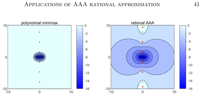
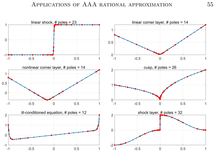
- For functions with branch points on the approximation domain, rational approximations converge root-exponentially, while polynomials converge only algebraically; the paper reports cases where degrees in the hundreds replace degrees in the millions.
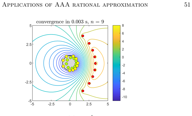
- Poles and zeros of a meromorphic function can be recovered from samples away from the singularities, often with accuracy that extends well beyond the data set, enabling fast singularity location in ODE, PDE, and scattering problems.
- Numerical analytic continuation by rational approximation can extend a function beyond its data domain by roughly one wavelength of its oscillatory behaviour, with the number of wavelengths growing with the working precision.
- Quadrature rules can be viewed as rational approximations of a Cauchy transform, so AAA can generate quadrature formulas adapted to arbitrary contours and weight functions; the paper shows classical Gauss-type rules reproduced this way.
- For model order reduction, a transfer function of degree 1000 can be reduced to degree about 30 by fitting samples on the imaginary axis, with ten-digit accuracy.
Reading between the lines
- If AAA's near-best behaviour is as general as the examples suggest, numerical libraries that currently rely on polynomial spectral methods could switch to AAA-based rational methods for stiff or singular problems, with order-of-magnitude reductions in degree and no loss of accuracy.
- The roughly linear relation between working precision and the number of wavelengths of analytic continuation suggests a testable law: doubling the digits should roughly double the achievable extension distance; a systematic experiment across functions with known singularities could turn the one-wavelength principle into a theorem or refute it.
- The equivalence between quadrature nodes and poles of rational approximations of a Cauchy transform suggests a design principle: for any new kernel or contour, one can derive a quadrature rule by solving a rational approximation problem, which may be more direct than constructing conformal maps.
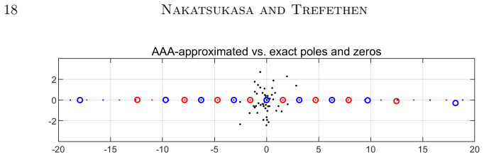
- The paper's own Burgers example—where AAA poles agree with exact poles only near the real axis—implies that pole-based singularity inference has a finite horizon; a careful study of how this horizon depends on tolerance, sample clustering, and singularity strength would delineate where AAA can be trusted.
Editorial analysis
A structured set of objections, weighed in public.
Referee Report
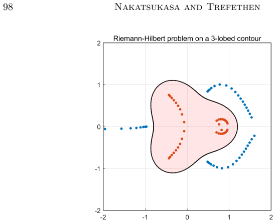
Summary. This invited review demonstrates the AAA algorithm for rational approximation across 26 areas of numerical analysis, including function approximation, pole/zero and branch-point location, differentiation and integration, analytic continuation, ODE/PDE extension into the complex plane, eigenvalues and resonances, model order reduction, Zolotarev sign and ratio problems, quadrature, Cauchy/Wiener-Hopf/Riemann–Hilbert problems, and conformal mapping. The paper is experiment-driven: each section contains MATLAB snippets, figures, and a candid discussion of what is known, conjectured, or open. The central claim, stated in Section 1, is that AAA-type rational approximation is a fast, near-best, general-purpose tool that outperforms polynomial methods for functions with singularities and for extrapolation. The authors are explicit that parts of the theory are missing, and they list twenty open problems.
Significance. If the demonstrations are correct, this is an important and timely review that makes a strong case for rational approximation as a routine numerical tool. The paper's strengths include reproducible code snippets, external analytic checks (the two-disk Zolotarev ratio is within 0.1% of the known value in Section 21; resonances in the closed disk match Bessel roots in Section 16), and unusually candid disclosure of limitations and failure modes, such as the Section 14 pole discrepancy and the Section 20 sign-problem difficulties. The review will be a valuable resource for practitioners and researchers. However, the broad-utility thesis is conditional on the empirical reliability of AAA's poles and extrapolated values, and two of the paper's own examples show that this reliability has limits. Those limits are acknowledged but not quantified, and they affect several of the showcased applications, so the manuscript would benefit from a dedicated discussion of reliability and diagnostics.
major comments (3)
- [Section 14; also Sections 4, 16–18, 22] The manuscript reproduces a VandenHeuvel et al. experiment in which AAA poles for a Burgers solution differ completely from the exact poles beyond the pair closest to the real axis, despite a 1e-13 fit on the real axis. This is a documented counterexample to the inference that a good data fit implies correct singularity structure—an inference used in pole/zero finding (Section 4), resonance and eigenvalue computation via poles of scalarized resolvents (Sections 16–18), and quadrature-node interpretation (Section 22). The paper warns about this in Section 14 but does not provide a diagnostic, a frequency estimate, or a stability check. Since the broad-utility claim is supported by selected examples, this gap is load-bearing. I ask for a short 'reliability of pole extraction' discussion: for instance, sensitivity of computed poles to sample perturbation, or an a posteriori consistency test
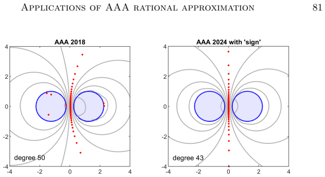
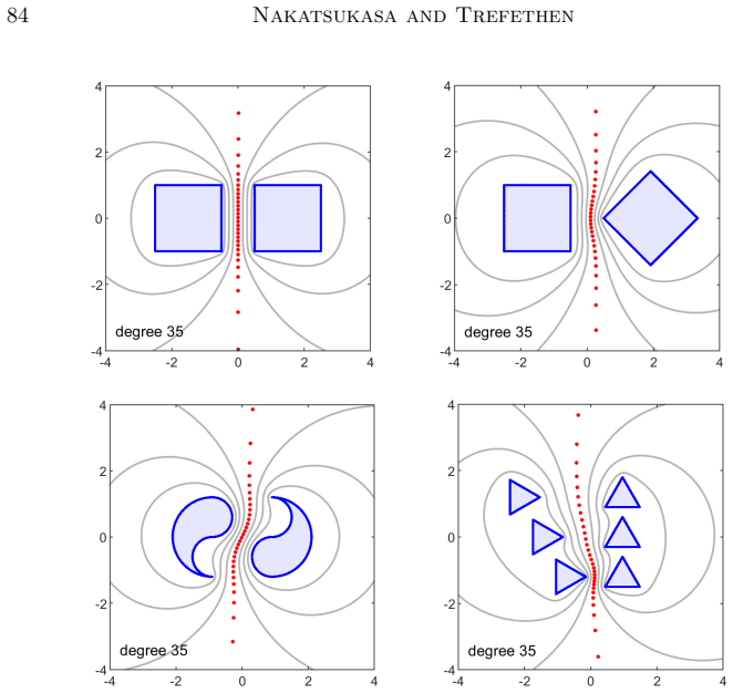
- [Section 20, Eqs. (20.2)–(20.3); Section 21] The paper states that standard AAA 'almost invariably runs into trouble' on Zolotarev sign problems, and the 'sign' and 'damping' fixes are explicitly 'not bulletproof' and have no theoretical justification. The Zolotarev ratio problem of Section 21 is solved through these fixes, and the Batakci-spiral example is admitted to be 'only approximate' and not fully converged. Thus the paper's own headline examples in Sections 20–21, and their downstream applications (quadrature, MOR), are outside the regime of routine AAA reliability. Please add a quantitative statement of when the sign modification succeeds or fails (for example, over a small corpus of E/F geometries) and clarify which of the 26 applications inherit this caveat.
- [Section 10; Section 2] The paper's extrapolation claims are central, especially for analytic continuation and extension of ODE/PDE solutions into C. Yet Section 10's one-wavelength principle is explicitly a rule of thumb, not a theorem, and Section 2 states that no theorem ensures AAA is near-best in the relevant sense. The paper gives no general guidance beyond 'about one wavelength' for when extrapolated values can be trusted. Since Sections 13–15 and 24–28 build on continuation of computed solutions, this is a load-bearing heuristic. Please either provide a more precise accuracy-versus-distance tradeoff or mark the affected applications as heuristic in the relevant sections.
minor comments (4)
- [Section 21, code after Eq. (21.7)] The code defines rstar without the factor sqrt(sigma) that appears in Eq. (21.4). This is harmless for pole/zero plots but should be noted if the normalized value is needed.
- [Section 16, table] The entry 'same' for mode 3 in the closed-circle column would be clearer if the numerical value 3.8317060 were repeated.
- [Section 12, Theorem 12.1] The theorem is attributed to Stahl (1989, Lemma 2) but no proof or precise statement of the specialization is given. Adding a sentence on how the stated version follows would help readers.
- [Section 4, Eq. (4.1)] The display of the generalized eigenvalue problem is visually hard to parse in the arXiv version; a clearer matrix layout or a reference to Corless (2004) with the exact eigenvalue problem would improve readability.
Circularity Check
No significant circularity: the paper's demonstrations are largely independent numerical experiments verified against exact or external data; self-citations are references to documented algorithms and prior work, not load-bearing reductions.
full rationale
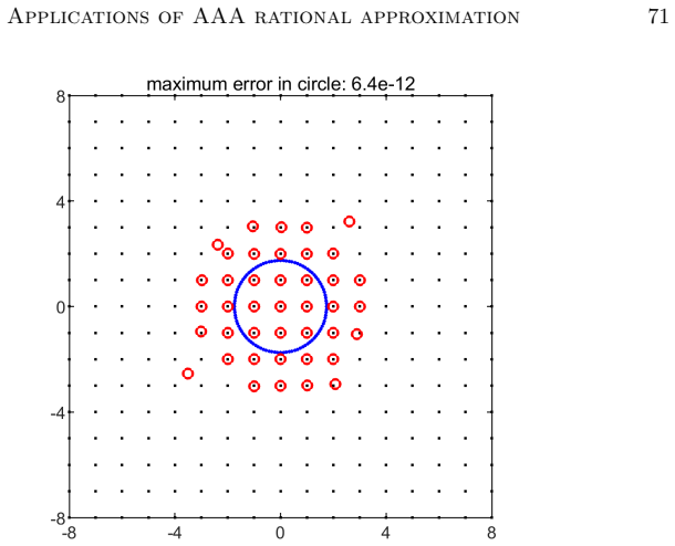
The central claim is an empirical advocacy thesis: AAA rational approximation is fast, flexible, and near-best across many applications. The supporting evidence is not a derivation that assumes its conclusion. For example, Section 3 evaluates a AAA fit at z=2 and checks against the known value of tan(2)/tan(2); Section 4 compares computed poles and zeros of tan and zeta against the exact values; Section 17 checks eigenvalue poles against exactly known diagonal entries; Section 21 checks the Zolotarev ratio against the analytic value 2^-60 within 0.1%. Section 2 explicitly disclaims any theorem that AAA is near-best: "The true theoretical challenge of AAA approximation is to establish a theorem to ensure that, under appropriate assumptions, AAA finds not just accurate but near-best approximations." The paper also documents failures, notably Section 14's reproduction of VandenHeuvel et al. showing AAA pole sets for a Burgers solution differing from exact poles while the functions agree to 10^-13 on the real axis. This is a reliability limitation, not a circular step. The many self-citations (Nakatsukasa-Sète-Trefethen 2018; Trefethen-Wilber 2025; Bruno-Santana-Trefethen submitted; Horning-Trefethen submitted; Driscoll-Nakatsukasa-Trefethen 2024) point to documented algorithms and prior work whose contents are independently reproducible (MATLAB/Chebfun code, external verification, and mathematical derivations reproduced in the text, e.g. Section 22 equations (22.4)-(22.9)). None of these citations is used in place of a missing derivation, and the central experimental results are checked against external benchmarks rather than against the paper's own fit. No claim is a fitted input renamed as a prediction; no ansatz is smuggled in via citation; no uniqueness theorem from the authors is invoked to forbid alternatives, and the paper explicitly acknowledges other methods such as Thiele continued fractions. The limitation flagged in Section 14 weakens the pole-inference applications but does not make the paper's reasoning circular.
Assumptions & free parameters
free parameters (4)
- AAA stopping tolerance =
10^-13 default; 10^-7 to 10^-10 in several experiments
- Rational degree n or degree limits =
varies (e.g., 30, 35, 80, 150)
- Lawson iteration count and damping factor delta =
20-600 steps; delta = 0.95, 0.75
- Sample set Z (geometry and size) =
chosen per experiment (50-3000 points)
assumptions (6)
- standard math Standard complex analysis: Cauchy integral formula, residue theorem, Sokhotski-Plemelj formulas, Schwarz reflection principle (Theorems 11.1-11.2)
- domain assumption Walsh Hermite integral formula (12.1)-(12.2) and the Gonchar-Stahl rho^2 2n+1 interpolation-point version (Theorem 12.1)
- ad hoc to paper AAA (as implemented in Chebfun aaa.m) genuinely achieves the reported accuracy, and sample-set convergence implies the claimed continuum accuracy
- domain assumption Istace-Thiran equivalence between Zolotarev sign and ratio problems (Theorem 21.1)
- domain assumption Known analytic benchmarks: two-disk Zolotarev solution (21.7)-(21.8) from Starke (1992); Bessel-root eigenvalues for the closed circular cavity (Section 16); Chapman's asymptotic formulas (16.3)-(16.5)
- domain assumption Numerical environment: IEEE double precision and correct behavior of MATLAB/Chebfun functions (aaa.m, minimax, chebfun)
Cite this review
Pith. "Pith review of Applications of AAA rational approximation." pith.science (2026). https://pith.science/paper/OH44KBYV
@misc{pith2026251016237,
  author       = {Pith},
  title        = {Pith review of: Applications of AAA rational approximation},
  year         = {2026},
  howpublished = {\url{https://pith.science/paper/OH44KBYV}},
  note         = {Machine review of arXiv:2510.16237}
}
read the original abstract
The AAA algorithm for rational approximation is employed to illustrate applications of rational functions all across numerical analysis.
Figures


Figures from the paper (61 more)

















Forward citations
Cited by 1 Pith paper
-
Rational Minimax Approximations for Matrix-Valued Functions: Existence, Optimality and Algorithms
Matrix-valued rational minimax approximants with a common denominator are proved to exist on dense point sets, with Kolmogorov/Ruttan optimality certificates and an equivalence to the m-d-Lawson dual conditions.
Reference graph
Works this paper leans on
-
[1]
Adcock and D
B. Adcock and D. Huybrechs (2019), Frames and numerical approximation,SIAM Rev.61, 443–473. B. Alpert, L. Greengard and T. Hagstrom (2000), Rapid evaluation of nonreflecting boundary kernels for time-domain wave propagation,SIAM J. Numer. Anal.37, 1138–1164. A. C. Antoulas and B. D. Q. Anderson (1986), On the scalar rational interpolation problem,IMA J. M...
2019
-
[3]
Bai and J
Z. Bai and J. Demmel (1998), Using the matrix sign function to compute invariant subspaces,SIAM J. Matrix Anal. Applics.19(1), 205–225. Z. Bai, J. Demmel and M. Gu (1997), An inverse free parallel spectral divide and conquer algorithm for nonhermitian eigenproblems,Numer. Math.76, 279–308. G. A. Baker, Jr. (1961), Application of the Pad´ e approximant met...
1998
-
[7]
S. J. Harris and N. R. McDonald (2025a), Modelling wildfire spread and spot- fire merger using conformal mapping and AAA-least squares methods,Environ. Model. Softw.185, 106303. S. J. Harris and N. R. McDonald (2025b), Vortex equilibria using least-squares methods,Theor. Comput. Fluid Dyn.39, 1–17. S. J. Harris, R. A. Palmer and N. R. McDonald (2025), Mod...
2025
-
[14]
M. C. Brennan, M. Embree and S. Gugercin (2023), Contour integral methods for nonlinear eigenvalue problems: A systems theoretic approach,SIAM Rev.65, 439–470. P. D. Brubeck and L. N. Trefethen (2022), Lightning Stokes solver,SIAM J. Sci. Comput.44, A1205–A1226. P. D. Brubeck, Y. Nakatsukasa and L. N. Trefethen (2021), Vandermonde with Arnoldi,SIAM Rev.63...
arXiv 2023
-
[16]
I. V. Gosea and S. G¨ uttel (2021), Algorithms for the rational approximation of matrix-valued functions,SIAM J. Sci. Comput.43, A3033–A3054. A. Greenbaum and L. N. Trefethen (1994), GMRES/CR and Arnoldi/Lanczos as matrix approximation problems,SIAM J. Sci. Comp.15, 359–368. S. Gugercin, A. C. Antoulas and C. Beattie (2008),H 2 model reduction for large- ...
2021
-
[21]
Applications of AAA rational approximation145 A. C. Ionita (2013), Lagrange rational interpolation and its applications to approx- imation of large-scale dynamical systems, PhD thesis, Rice University. M.-P. Istace and J.-P. Thiran (1993), On computing best complex rational approx- imants,Numerical Algorithms5, 299–308. M.-P. Istace and J.-P. Thiran (1995...
2013
-
[25]
L. N. Trefethen (to appear), Numerical conformal mapping,Notices of the AMS. L. N. Trefethen and J. A. C. Weideman (2014), The exponentially convergent trapezoidal rule,SIAM Rev.56, 385–458. L. N. Trefethen and H. D. Wilber (2025), Computation of Zolotarev rational func- tions,SIAM J. Sci. Comput.47, A2205–A2220. L. N. Trefethen, A. Birkisson and T. A. Dr...
2014
-
[36]
Platte, L
R. Platte, L. N. Trefethen and A. B. J. Kuijlaars (2011), Impossibility of fast stable approximation of analytic functions from equispaced samples,SIAM Rev. 53, 308–318. E. Polizzi (2009), Density-matrix-based algorithm for solving eigenvalue problems, Phys. Rev. B79, 115112–1–115112–6. C. Pozrikidis (1992),Boundary Integral and Singularity Methods for Li...
2011
Show all 16 references
-
[150]
L. N. Trefethen (2023), Numerical analytic continuation,Jpn. J. Ind. Appl. Math. 40, 1587–1636. L. N. Trefethen (2024), Polynomial and rational convergence rates for Laplace problems on planar domains,Proc. Roy. Soc. A480, 20240178. Applications of AAA rational approximation14...
2023
-
[283]
J. H. Curtiss (1962), Interpolation by harmonic polynomials,J. SIAM10, 709–736. P. J. Davis (1974),The Schwarz Function and its Applications, Math. Assoc. Amer. P. J. Davis and H. Pollak (1958), On the analytic continuation of mapping func- tions,Trans. AMS87, 198–225. E. Deck...
1962 arXiv
-
[1004]
MacMillen (2024), BaryRational.jl,github.com/macd/BaryRational.jl
D. MacMillen (2024), BaryRational.jl,github.com/macd/BaryRational.jl. MathWorks Inc. (2020), ‘RF Toolbox’,https://www.mathworks.com. T. Matsuda and Y. Nakatsukasa (2025), Polynomial approximation of noisy func- tions,Numer. Math.157, 1285–1311. S. W. McCue, C. J. Lustri, D. J....
2024 arXiv
-
[1236]
A. C. Rodriguez, L. Balicki and S. Gugercin (2023), The p-AAA algorithm for data-driven modeling of parametric dynamical systems,SIAM J. Sci. Comput. 45, A1332–A1358. V. Rokhlin (1990), Rapid solution of integral equations of scattering theory in two dimensions,J. Comput. Phys...
2023
-
[1671]
Boull´ e, A
N. Boull´ e, A. Herremans and D. Huybrechs (2024), Multivariate rational approx- imation of functions with curves of singularities,SIAM J. Sci. Comput.46, A3401–A3426. N. Boull´ e, Y. Nakatsukasa and A. Townsend (2020), Rational neural networks, Adv. Neural Info. Proc. Syst.33...
2024
-
[1821]
A. P. Austin, M. Krishnamoorthy, S. Leyffer, S. Mrenna, J. M¨ uller and H. Schulz (2021), Practical algorithms for multivariate rational approximation,Computer Phys. Commun.261, 107663. S. Axler (1986), Harmonic functions from a complex analysis viewpoint,Amer. Math. Monthly93...
2021
-
[2025]
T. A. Driscoll and Y. Zhou (2025), Greedy Thiele continued-fraction approximation on continuum domains in the complex plane,arXiv preprint arXiv:2510.07295. T. A. Driscoll, F. Bornemann and L. N. Trefethen (2008), The chebop system for automatic solution of differential equati...
2025
-
[2523]
S. J. Harris and N. R. McDonald (2023), Penguin huddling: a continuum model, Acta Appl. Math.185,
2023
Reviewed August 4, 2026 · model on record in the stance chip above.
Discussion (0). Continue with ORCID to comment.