REVIEW 4 major objections 6 minor 17 references
SITES: Solar Iterative Temperature Emission Solver for differential emission measure inversion of EUV observations
T0 review · 4 major / 6 minor · reviewed 2026-08-14 · deepseek-v4-flash
Pith's one-line read SITES recovers coronal temperature structure from EUV images using a simple iterative solver.
desk verdict A well-designed DEM solver with honest tests, but the printed Eq. 4 is wrong—the paper's own results cannot follow from the stated algorithm without a fix and released code. read the letter →
The pith
A machine-rendered reading of the paper's core claim, the machinery that carries it, and where it could break.
The reading
What carries the argument
The core object is the relative temperature response $S_{ij} = w_i R_{ij} / (\sum_i w_i R_{ij})$, built from each channel's response function $R_{ij}$ weighted by measurement and calibration errors. Equation (4) converts observed intensities $I_i$ into an initial DEM by distributing each channel's intensity across temperature according to $R_{ij}$, combining channels through $S_{ij}$, and convolving with a narrow Gaussian in logarithmic temperature. The iteration then computes modelled intensities $M_i = \sum_j D_j R_{ij} \Delta T_j$, feeds the residual $I_i - M_i$ back through the same redistribution, and clips negative DEM values to zero, stopping when the weighted mean absolute residual falls below a threshold such as 4%. This iterative residual-correction loop, together with the single smoothing width, is what carries the whole argument.
What would settle it
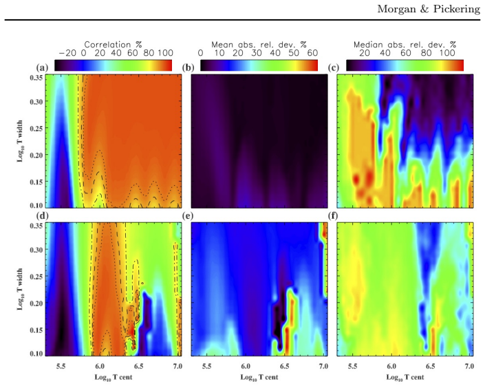
A blind benchmark on synthetic AIA data spanning central temperatures from log T = 5.7 to 7.0 and widths from log T = 0.1 to 0.35, with Poisson noise added, would settle the accuracy claim: the central claim is wrong if SITES systematically shows input–output DEM correlations below 95% inside the region the paper marks as reliable, or if its measured residuals do not fall below the convergence threshold it reports.
Extended reading notes
Core claim
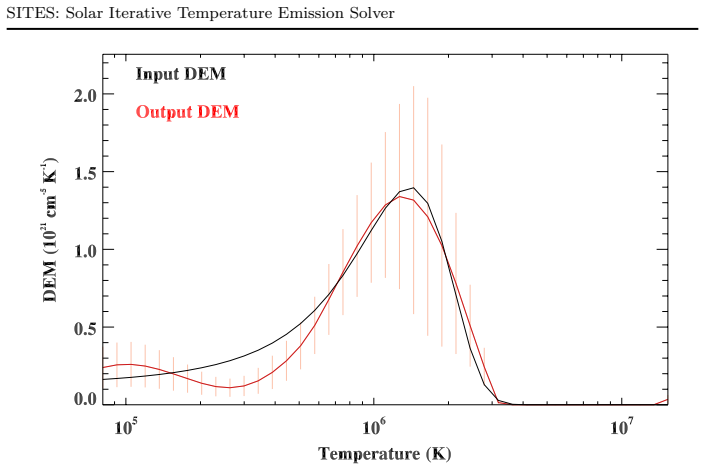
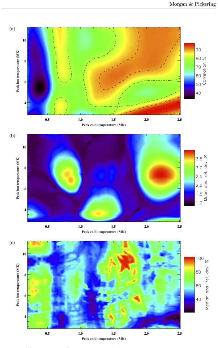
The central claim is that SITES reconstructs a DEM by first spreading each measured intensity across temperature in proportion to that channel's response function, combining the channels with inverse-noise weights, then repeatedly adding DEM corrections built from the residual intensities until the weighted residuals drop below a threshold. In tests on synthetic AIA observations, the recovered DEMs correlate at 95–98% with the input model across broad ranges of peak temperature and width, with median deviations around 12–26% for representative single- and double-Gaussian targets. The method is deliberately minimal: the only user-selected parameter is the width of a Gaussian smoothing kernel in logarithmic temperature, with positivity enforced by thresholding. The paper concedes two limits—very narrow DEM peaks are not well recovered at any temperature, and temperatures below about 0.5 MK are not reliable with AIA data—and argues these limits follow from the instrument's broad response functions rather than from the solver. On identical synthetic inputs, SITES matches or outperforms both a sparse-basis method and a Tikhonov-regularized method used as benchmarks, while running at roughly a thousand DEMs per second at the routinely used convergence threshold.
Load-bearing premise
The reconstruction inherits whatever bias lives in the AIA temperature response functions; if those functions are wrong, the iterative fitting cannot correct it, because the method only tries to match intensities computed with the same functions.
Editorial extensions
If this is right
- Long time-series of AIA full-disk DEM maps become practical: at about 1,000 profiles per second, a full 4k disk can be processed in minutes to hours rather than days.
- Multi-channel EUV instruments beyond AIA can use the same solver directly, provided their temperature response functions and error estimates are known.
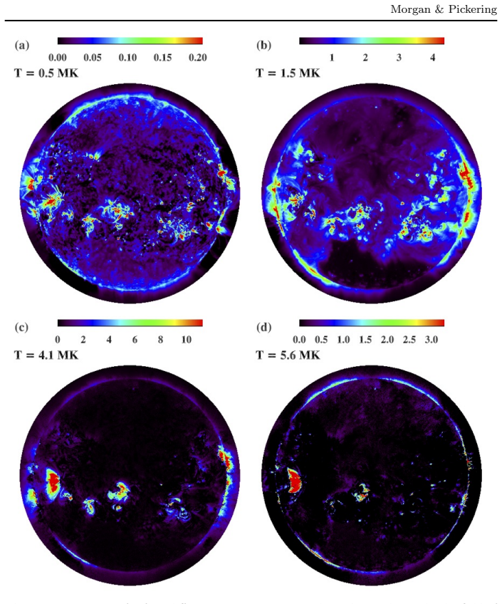
- The fractional emission measure visualization gives a standard, normalized way to compare which temperatures dominate in coronal holes, quiet Sun, and active region cores, independent of total emission.
- The method's reliance on a single smoothing parameter makes it easier to reproduce and less dependent on analyst choices than methods with several tuning parameters.
- Broad multithermal coronal structures are the natural target; narrow isothermal-like plasmas and sub-0.5 MK material should be interpreted with caution.
Reading between the lines
- A direct extension is to feed SITES DEMs into rotational tomography: using multiple viewpoints would address the line-of-sight bias the paper notes for off-limb regions, and could also regularize narrow peaks.
- The error bars from Equation (6) omit smoothing and iteration effects; the paper's own low-signal test shows underestimated uncertainty above ~2 MK, so users should treat those error bars as optimistic in faint regions.
- The real 0.5 MK floor is a property of AIA's response functions, not of the algorithm; applying SITES to observations with stronger low-temperature sensitivity would likely push the useful range lower, a testable prediction.
- Because the iteration is a residual-correction map with positivity clipping, it should be possible to prove convergence conditions, which might let future users choose thresholds automatically rather than by trial.
Signed reviews
Editorial analysis
A structured set of objections, weighed in public.
Referee Report
Summary. The paper presents SITES, an iterative differential emission measure (DEM) inversion method for AIA EUV observations. The method builds an initial DEM by backprojecting each channel's intensity across temperature according to the channel response, then iteratively updates the DEM using intensity residuals with positivity and smoothing constraints. The authors test SITES on synthetic DEMs (single and multi-Gaussian, with and without noise), measure its speed, compare it with the methods of Cheung et al. (2015) and Hannah & Kontar (2012), and apply it to full-disk AIA data. They also introduce a fractional emission measure (FEM) visualization. The central claims are that SITES is simple, fast (about 1000 DEMs per second), non-subjective apart from one smoothing parameter, and accurate for broad DEMs above ~0.5 MK, while performing poorly on narrow peaks and low-temperature DEMs.
Significance. If the method works as described, it is a useful addition to the DEM inversion toolbox: the synthetic validation is extensive, the authors explicitly characterize the failure modes (narrow peaks, temperatures below ~0.5 MK), and the uncertainty estimate is checked against Monte Carlo repetitions. The FEM visualization is a simple and effective idea for comparing temperature regimes across coronal structures. The speed and simplicity could make it practical for large AIA datasets. However, the central equation of the method as printed is not intensity-preserving, so the validation presented in Section 3 cannot be reproduced from the manuscript as written; this is a load-bearing issue that must be corrected before the results can be credited.
major comments (4)
- [Section 2, Eq. (4)] As printed, Eq. (4) cannot be the backprojection used in the paper. The per-channel term is I_i/(R_ij ΔT_j) times Σ_j (R_ij ΔT_j)^2, so for a single channel the forward-modeled intensity obtained by summing D_j R_ij ΔT_j over j is n_t I_i Σ_j (R_ij ΔT_j)^2, not I_i. The expression is also dimensionally inconsistent: it carries units of intensity times response, not DEM. The standard intensity-preserving backprojection would be I_i R_ij ΔT_j / Σ_j (R_ij ΔT_j)^2, with the sum in the denominator. Because no derivation or public code is provided, the text alone does not specify a valid, reproducible algorithm, and the convergence, timing, and comparison results in Section 3 cannot be traced to the stated equation. Please correct Eq. (4), provide a derivation, and state explicitly which expression was used in the synthetic tests.
- [Section 2, Eq. (6)] The quantity d_j defined in Eq. (6) is dimensionless: it is the square root of a weighted sum of squared relative errors (σ_i/I_i)^2 and ε_i^2. Yet it is presented as 'the final DEM uncertainty' and is compared in Figures 2, 9, and 10 to the absolute spread of DEMs, which has units cm^-5 K^-1. If d_j is intended as a relative uncertainty, this must be stated and the plotted error bars must be multiplied by the DEM value; if it is intended as an absolute error, the equation is incomplete. This issue directly affects the validation claim in Section 3.4 that the uncertainty estimate 'reflects well the true variation of the output DEMs.'
- [Sections 1 and 5] The claim that SITES is 'non-subjective' and that the smoothing kernel width is the only parameter affecting the result is overstated. The kernel width is chosen by trial and error with the criterion that it be minimal 'whilst still resulting in smooth DEMs', which is a subjective regularization choice. Moreover, Section 3.3 shows that the convergence threshold also affects both the fitted intensities and the output DEM (Figure 8a), so the convergence threshold is another parameter that influences the result. The non-subjectivity claim should be qualified to 'a single tunable regularization parameter plus a stopping criterion', and the dependence on the convergence threshold should be acknowledged in the summary.
- [Section 3.3] The text in Section 3.3 refers to a 'complex 3-Gaussian plus background' DEM, while the complex test in Section 3.2 is explicitly defined as two Gaussian peaks plus a constant background. This inconsistency makes it unclear which model was used for the speed and convergence-threshold tests. Please correct the description so that the number of Gaussians matches the actual test DEM.
minor comments (6)
- [Section 3.5] There is a typo: 'perofrmance' should be 'performance'.
- [Section 4.1] There is a typo: 'measurmeent' should be 'measurement'.
- [Section 2] The sentence following Eq. (4) says that integrating the individual DEMs over temperature would result in exactly the observed intensities; this statement is only true for the corrected form of the equation, not for the printed form. Please move this explanatory sentence next to the corrected equation.
- [General] The software is only available 'by email request to the authors'. For reproducibility, especially given the error in Eq. (4), please consider providing a version-controlled repository or a complete pseudocode listing that includes the exact update rule and convergence criterion.
- [Section 3.5] In the comparison with SMI, the plots show EM rather than DEM for the SMI output, and the text notes this in the caption; however, the y-axis labels are not visible in Figures 11a and 11b. Please ensure the figure axes make the EM/DEM distinction explicit.
- [Abstract] The abstract states 'about 1000 DEMs per second', but Section 3.3 reports this speed at a convergence threshold of 4%. The threshold dependence is shown in Figure 8b, so the abstract should either quote the speed with the associated threshold or mention that the speed is threshold-dependent.
Circularity Check
No significant circularity: SITES is benchmarked against externally defined model DEMs; no parameter is fitted to the test targets, and the only self-citations are contextual.
full rationale
The central inversion update (Eq. 4) and forward model (Eq. 5) are stated as independent definitions, and the method's adjustable smoothing kernel is explicitly a regularization choice: the paper says the width is found through trial and error with the criterion that the smoothing width is kept at a minimum 'whilst still resulting in smooth DEMs,' not by matching the benchmark DEMs. The Section 3 validation uses model DEMs defined by Eq. 7 and the two-Gaussian/background variants, compares the inversion to those targets through the independently defined correlation (Eq. 10) and deviation (Eq. 9), and compares SITES with the independent methods of Cheung et al. (2015) and Hannah & Kontar (2012) using identical response functions and synthetic measurements. The only self-citations (Morgan & Taroyan 2017 and Morgan & Druckmüller 2014) appear as background or image-processing context and do not carry the inversion argument. No fitted parameter is renamed as a prediction: the data-consistency residual is an iteration target, while the DEM-recovery claim is checked against externally constructed model DEMs, so the central results do not reduce to the method's own inputs.
Assumptions & free parameters
free parameters (2)
- Smoothing kernel width =
3.2 bins in logarithmic temperature
- Convergence threshold =
4% for real data (1% in tests)
assumptions (4)
- domain assumption The solar corona is optically thin in EUV, so measured intensities are line-of-sight integrals of the emission measure times temperature response.
- domain assumption The AIA temperature response functions Rij, computed from CHIANTI atomic data and EVE calibration, are accurate.
- domain assumption The plasma is in thermal equilibrium with Maxwell-Boltzmann electron distributions, so the DEM formalism applies.
- ad hoc to paper Positivity and smoothness are the only needed constraints to solve the underdetermined inversion.
Cite this review
Pith. "Pith review of SITES: Solar Iterative Temperature Emission Solver for differential emission measure inversion of EUV observations." pith.science (2026). https://pith.science/paper/OLD4SEBN
@misc{pith2026190807773,
  author       = {Pith},
  title        = {Pith review of: SITES: Solar Iterative Temperature Emission Solver for differential emission measure inversion of EUV observations},
  year         = {2026},
  howpublished = {\url{https://pith.science/paper/OLD4SEBN}},
  note         = {Machine review of arXiv:1908.07773}
}
read the original abstract
Extreme UltraViolet (EUV) images of the optically-thin solar corona in multiple spectral channels give information on the emission as a function of temperature through differential emission measure (DEM) inversions. The aim of this paper is to describe, test, and apply a new DEM method named the Solar Iterative Temperature Emission Solver (SITES). The method creates an initial DEM estimate through a direct redistribution of observed intensities across temperatures according to the temperature response function of the measurement, and iteratively improves on this estimate through calculation of intensity residuals. It is simple in concept and implementation, is non-subjective in the sense that no prior constraints are placed on the solutions other than positivity and smoothness, and can process a thousand DEMs per second on a standard desktop computer. The resulting DEMs replicate model DEMs well in tests on Atmospheric Imaging Assembly (AIA) synthetic data. The same tests show that SITES performs less well on very narrow DEM peaks, and should not be used for temperature diagnostics below ~0.5MK in the case of AIA observations. The SITES accuracy of inversion compares well with two other established methods. A simple yet powerful new method to visualise DEM maps is introduced, based on a fractional emission measure (FEM). Applied to a set of AIA full-disk images, the SITES method and FEM visualisation show very effectively the dominance of certain temperature regimes in different large-scale coronal structures. The method can easily be adapted for any multi-channel observations of optically-thin plasma and, given its simplicity and efficiency, will facilitate the processing of large existing and future datasets.
Figures


Figures from the paper (14 more)







Reference graph
Works this paper leans on
-
[1]
: 2005 , Physics of the Solar Corona
bbook Aschwanden , M.J. : 2005 , Physics of the Solar Corona. An Introduction with Problems and Solutions (2nd edition) . bbook
work page 2005
-
[2]
barticle Boerner , P.F. , Testa , P. , Warren , H. , Weber , M.A. , Schrijver , C.J. : 2014 , Photometric and thermal cross-calibration of solar euv instruments . Solar Physics 289 ( 6 ), 2377 \,--\, 2397 . doi: 10.1007/s11207-013-0452-z . https://doi.org/10.1007/s11207-013-0452-z . barticle
-
[3]
barticle Cheung , M.C.M. , Boerner , P. , Schrijver , C.J. , Testa , P. , Chen , F. , Peter , H. , Malanushenko , A. : 2015 , Thermal Diagnostics with the Atmospheric Imaging Assembly on board the Solar Dynamics Observatory: A Validated Method for Differential Emission Measure Inversions . 807 , 143 . doi: 10.1088/0004-637X/807/2/143 . barticle
-
[4]
: 2013 , The multi-thermal emission in solar active regions
barticle Del Zanna , G. : 2013 , The multi-thermal emission in solar active regions . 558 , A73 . doi: 10.1051/0004-6361/201321653 . barticle
-
[5]
barticle Dere , K.P. , Landi , E. , Mason , H.E. , Monsignori Fossi , B.C. , Young , P.R. : 1997 , CHIANTI - an atomic database for emission lines . 125 , 149 \,--\, 173 . doi: 10.1051/aas:1997368 . barticle
-
[6]
: 2009 , Phase Correlation Method for the Alignment of Total Solar Eclipse Images
barticle Druckm \"u ller , M. : 2009 , Phase Correlation Method for the Alignment of Total Solar Eclipse Images . 706 , 1605 \,--\, 1608 . doi: 10.1088/0004-637X/706/2/1605 . barticle
-
[7]
bchapter Fisher , G.H. , Welsch , B.T. : 2008 , FLCT: A Fast, Efficient Method for Performing Local Correlation Tracking . In: Howe , R. , Komm , R.W. , Balasubramaniam , K.S. , Petrie , G.J.D. (eds.) Subsurface and Atmospheric Influences on Solar Activity , Astronomical Society of the Pacific Conference Series 383 , 373 . bchapter
work page 2008
-
[8]
barticle Hahn , M. , Savin , D.W. : 2014 , Evidence for Wave Heating of the Quiet-Sun Corona . 795 , 111 . doi: 10.1088/0004-637X/795/2/111 . barticle
Show all 17 references
-
[9]
, Landi , E
barticle Hahn , M. , Landi , E. , Savin , D.W. : 2011 , Differential Emission Measure Analysis of a Polar Coronal Hole during the Solar Minimum in 2007 . 736 , 101 . doi: 10.1088/0004-637X/736/2/101 . barticle
2011 doi
-
[10]
, Kontar , E.P
barticle Hannah , I.G. , Kontar , E.P. : 2012 , Differential emission measures from the regularized inversion of Hinode and SDO data . 539 , A146 . doi: 10.1051/0004-6361/201117576 . barticle
2012 doi
-
[11]
, Del Zanna , G
barticle Landi , E. , Del Zanna , G. , Young , P.R. , Dere , K.P. , Mason , H.E. : 2012 , CHIANTI - An Atomic Database for Emission Lines. XII. Version 7 of the Database . 744 , 99 . doi: 10.1088/0004-637X/744/2/99 . barticle
2012 doi
-
[12]
, Dzif c \'a kov \'a , E
barticle Mackovjak , S . , Dzif c \'a kov \'a , E. , Dud \' k , J. : 2014 , Differential emission measure analysis of active region cores and quiet Sun for the non-Maxwellian -distributions . 564 , A130 . doi: 10.1051/0004-6361/201323054 . barticle
2014 doi
-
[13]
, Taroyan , Y
barticle Morgan , H. , Taroyan , Y. : 2017 , Global conditions in the solar corona from 2010 to 2017 . Science Advances 3 ( 7 ). doi: 10.1126/sciadv.1602056 . https://advances.sciencemag.org/content/3/7/e1602056 . barticle
2017 doi
-
[14]
, Druckm \"u ller , M
barticle Morgan , H. , Druckm \"u ller , M. : 2014 , Multi-scale gaussian normalization for solar image processing . Solar Physics 289 ( 8 ), 2945 \,--\, 2955 . doi: 10.1007/s11207-014-0523-9 . https://doi.org/10.1007/s11207-014-0523-9 . barticle
2014 doi
-
[15]
, V \' a squez , A.M
barticle Nuevo , F.A. , V \' a squez , A.M. , Landi , E. , Frazin , R. : 2015 , MULTIMODAL DIFFERENTIAL EMISSION MEASURE IN THE SOLAR CORONA . The Astrophysical Journal 811 ( 2 ), 128 . doi: 10.1088/0004-637X/811/2/128 . https://doi.org/10.1088/0004-637x/811/2/128 . barticle
2015 doi
-
[16]
, Kankelborg , C
barticle Plowman , J. , Kankelborg , C. , Martens , P. : 2013 , Fast Differential Emission Measure Inversion of Solar Coronal Data . 771 , 2 . doi: 10.1088/0004-637X/771/1/2 . barticle
2013 doi
-
[17]
, Schmelz , J.T
barticle Weber , M.A. , Schmelz , J.T. , DeLuca , E.E. , Roames , J.K. : 2005 , Isothermal Bias of the ``Filter Ratio'' Method for Observations of Multithermal Plasma . 635 , 101 \,--\, 104 . doi: 10.1086/499125 . barticle
2005 doi
Reviewed August 14, 2026 · model on record in the stance chip above.
Discussion (0). Continue with ORCID to comment.