REVIEW 5 major objections 5 minor 58 references
Non-stop Variability of Sgr A* using JWST at 2.1 and 4.8 micron Wavelengths: Evidence for Distinct Populations of Faint and Bright Variable Emission
T0 review · 5 major / 5 minor · reviewed 2026-08-10 · deepseek-v4-flash
Pith's one-line read JWST observations of Sgr A* at 2.1 and 4.8 microns show its near-infrared emission flickers non-stop, with faint and bright variable components that have distinct spectral indices and a 3–40 second lag between the two bands.
desk verdict Solid JWST light curves convincingly show Sgr A* is never quiet in the NIR; the two-population spectral-index split and the 3–40 s lag need stronger statistical and background treatment before carrying the physical claims. read the letter →
The pith
A machine-rendered reading of the paper's core claim, the machinery that carries it, and where it could break.
The reading
What carries the argument
The central machinery is simultaneous NIRCam F210M and F480M photometry of Sgr A* with astrometric registration to ALMA 230 GHz images and per-epoch background subtraction, combined with (1) broken power-law fits to temporal power spectra, (2) broken linear fits to the 4.8-versus-2.1 µm flux-flux relation whose slope change marks the boundary between faint and bright populations, and (3) an age-stratified synchrotron model in which electrons are injected with an $E^{-2}$ spectrum and upper cutoff energy $E_c$, cool in a constant magnetic field $B$, and produce optically thin emission at the two NIR frequencies. The model's free parameters allow the observed loops and lags to be reproduced, yielding estimates of $B$ and $E_c$.
What would settle it
Measure the actual 4.8 µm stellar contamination independently, for example from high-resolution spectroscopy or a stellar-PSF model of S0-2, S24, and S29 at the observed epochs; if the true contamination exceeds the adopted background by more than about 2 mJy, the faint positive spectral indices disappear and the claimed two-population split in spectral index collapses.
Extended reading notes
Core claim
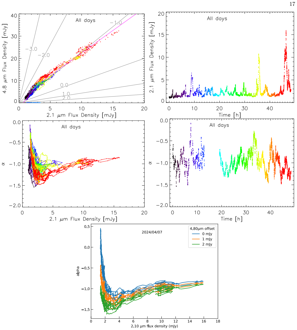
On its own terms, the paper establishes that Sgr A*'s near-infrared light curves, observed simultaneously at 2.1 and 4.8 µm with JWST NIRCam over seven epochs in 2023–2024, show continuous variability on timescales from seconds to hours in every epoch, with the pedestal level itself changing from day to day and year to year. The flux-flux correlation has a break near 3 mJy at 2.1 µm: fainter emission has spectral index $\alpha \approx -1.58$, brighter emission $\alpha \approx -0.85$, and the flux histogram is best described by two log-normal components. Cross-correlation reveals a 3–40 s lag of 4.8 µm behind 2.1 µm, and each flare traces a counterclockwise loop in spectral-index versus flux space. The paper interprets the loops as synchrotron cooling in an evolving, age-stratified electron population and derives magnetic field strengths of 40–90 G and cutoff energies of 420–720 MeV.
Load-bearing premise
The 4.8 micron background subtraction—including contamination from S0-2, S24, S29, and diffuse emission—is correct to within about 1–2 mJy; the paper shows that raising that background by 1–2 mJy erases the positive spectral indices of the faint emission, so the two-population spectral split depends on it.
Editorial extensions
If this is right
- If the non-stop variability claim is correct, there is no steady quiescent near-infrared component from Sgr A*, so models must explain an always-on flickering process rather than flares superimposed on a stable baseline.
- The ~3 mJy break in the flux-flux slope and the dual log-normal flux histogram imply two distinct particle populations: a faint steep-spectrum component and a bright shallow-spectrum flare component.
- The 3–40 s lag of 4.8 µm behind 2.1 µm, together with the counterclockwise spectral-index loops, implies synchrotron cooling in fields of 40–90 G with upper cutoff energies of 420–720 MeV.
- Sub-minute flux changes—up to a factor of two in about 1.4 minutes—place the emitting region at horizon scales of a few gravitational radii, linking the infrared variability to the inner accretion flow.
- The epoch-to-epoch pedestal changes by roughly a factor of two, showing long-term variability on daily, monthly, and yearly timescales that any complete model of Sgr A* must reproduce.
Reading between the lines
- If the two-population picture holds, future simultaneous two-band JWST observations could test whether the pedestal level predicts the amplitude or rate of bright flares; the paper notes a qualitative correlation between strong flaring and elevated pedestal but does not quantify it.
- Because the positive spectral indices of faint emission depend on a 4.8 µm background that is uncertain by 1–2 mJy, deeper imaging that resolves S0-2, S24, and S29 could either confirm the faint-component spectral index or show it is an artifact.
- The 3–40 s lag may be a general signature of synchrotron cooling in accreting black holes; if the lag scales with black hole mass, similar simultaneous two-band monitoring could constrain magnetic field strengths in other galactic nuclei.
- A direct test of the non-stop variability claim would be a longer, gap-free observation at 2.1 µm alone: if a true quiescent floor ever appears, the 'always fluctuating' interpretation would need revision.
Signed reviews
Editorial analysis
A structured set of objections, weighed in public.
Referee Report
Summary. This paper presents JWST/NIRCam photometry of Sgr A* in the F210M and F480M filters over seven epochs from April 2023 to April 2024, totaling roughly 48 h of nearly continuous monitoring. The authors report correlated variability at 2.1 and 4.8 micron in all epochs, continuous short-timescale (seconds-to-minute) fluctuations with no detected truly steady quiescent level, epoch-to-epoch changes in the underlying pedestal, a break in the flux-flux relation near 3 mJy at 2.1 micron, two spectral-index regimes (steep for faint, shallow for bright), 3-40 s lags of 4.8 micron relative to 2.1 micron, counterclockwise loops in spectral-index versus flux diagrams, and synchrotron flare modeling that yields magnetic field strengths of roughly 40-90 G and cutoff energies of 420-720 MeV. The data processing is described in unusual detail, with MAST-archived data, ALMA-based astrometric registration, reference-star noise checks, and explicit saturation-timing corrections.
Significance. The strongest claim, that Sgr A* is essentially always varying in the near-infrared rather than flaring atop a steady baseline, is well supported by the data presented: the reference stars are stable to their noise, the two bands vary in a correlated manner, and the variability amplitude is far above the photometric noise. If the spectral-index bimodality, short time delays, and magnetic-field estimates survive further scrutiny, this dataset will provide valuable new constraints on particle acceleration and cooling in the inner accretion flow. The openness of the data and the detailed treatment of systematic backgrounds are strengths. The remaining concerns are about the statistical support for several derived claims and about whether those claims are robust to the stated systematic uncertainties.
major comments (5)
- [§3.3, Table 6, Fig. 7e] The two-population spectral-index decomposition is not robust to the adopted 4.8 micron background. The paper states in §3.3 that increasing the 4.8 micron background by 1-2 mJy makes the positive spectral indices of the faint emission disappear. The slopes a± in the flux-flux plane are offset-independent, but the conversion to α− and α+ and the quoted values in Table 6 depend on the assumed background. Please propagate the estimated 1-2 mJy background uncertainty through to α−, α+, and S0, and show explicitly how the claimed bimodality and the loop interpretation change within that allowed range. As written, the title claim of distinct faint and bright populations is not yet established.
- [§3.4, Figs. 7-8] The reported 3-40 s inter-band delays are comparable to or shorter than the 18-46 s sampling cadence. The 4.8 micron data are interpolated onto the 2.1 micron grid, and the cross-correlation is applied to strongly correlated red-noise light curves, which can produce nonzero CCF peaks by chance. No confidence intervals, bootstrap/permutation significance levels, or null-hypothesis tests are reported. The authors should provide a significance estimate for each delay and demonstrate that the delays are not artifacts of the interpolation or of the saturation timing correction described in §2.2.
- [§3.2, Appendix A] The low-frequency break f0 reported in Table 5 may be systematically affected by the pedestal-removal procedure. Appendix A describes 4th-degree polynomial fits that are constrained to lie below the light curve; if these fits (or equivalent detrending) are removed before computing the power spectra, low-frequency power is suppressed by construction and the inferred f0 would not be intrinsic. The manuscript should state explicitly whether the PSDs are computed on raw or detrended light curves, and it should validate the f0 and n recovery using synthetic light curves with known power spectra processed through the same pedestal procedure. The Monte Carlo uncertainties in Table 5 do not include this systematic.
- [§3.1.5, Table 3] The claim of a bimodal flux distribution is not statistically quantified. Table 3 lists χ2 values but no degrees of freedom, reduced χ2, or model-selection criterion. At 4.8 micron the two-log-normal fit (χ2=82.11) is only slightly better than the log-normal-plus-power-law fit (χ2=85.77), despite the latter using a different functional form, and at 2.1 micron the log-normal-plus-power-law is preferred. The identification of two populations should be supported by a likelihood-ratio or information-criterion comparison that accounts for the number of parameters and for the small number of bright points.
- [§4.1, Appendix D, Table 7] The synchrotron model is described as having six free parameters (B, Q0, Ec, t0, t1, t2), but the fits in Table 7 also vary β1 and β2, giving eight parameters per flare. Fitting two light curves with eight parameters for each of five flares is likely to be strongly degenerate, so the quoted B=38-92 G and Ec=424-736 MeV ranges may not be meaningful as a 'direct estimate'. Please report parameter covariances or corner plots, specify whether the ranges are joint confidence intervals or merely the spread of best-fit values, and discuss how the assumed E^-2 injection spectrum and fixed E1=2 MeV affect the inferred B.
minor comments (5)
- [§3.1.5] The text refers to Table 3 for the mean, median, and sigma fluxes, but these quantities appear in Table 4; Table 3 contains the flux-distribution fit parameters.
- [References] The text cites 'Dodds-Eden et al. (1999)' in several places, but the bibliography lists Dodds-Eden et al. (2009); the year should be corrected consistently.
- [Fig. 7e caption and §3.3] The Figure 7e caption says the 4.8 micron subtracted background is reduced by 1 and 2 mJy, while §3.3 says it is increased by 1 and 2 mJy; these statements need to be reconciled.
- [Fig. 6 caption] The caption contains 'log-term quiescent variability'; this should be 'long-term'.
- [§2.4] The sentence about S24 and S29 spilling 'more flux in 2004 compared to 2003' appears to be a typo for 2024 and 2023.
Circularity Check
No significant circularity: the non-stop variability claim is anchored to stable reference-star photometry and two-band correlation, and the magnetic-field/cutoff values are explicit model fits rather than independent predictions.
full rationale
The central claim that Sgr A* is continuously variable is supported by data-internal controls: the reference star S0-17 is stable ('the fluxes are very stable, and flat with a flux density ... of 0.409 ± 0.001 mJy and 4.44 ± 0.02 mJy'), while Sgr A* fluctuates at both wavelengths in all epochs, and the 2.1/4.8 µm variations are correlated. Astrometric registration uses external ALMA 230 GHz positions, providing an independent coordinate anchor. The 4.8 µm background uncertainty is openly tested: the paper shows that raising the assumed background by 1–2 mJy removes the positive spectral indices of faint emission, so the two-population spectral-index split is presented as background-sensitive rather than as a hidden assumption. The magnetic field strengths (38–92 G) and cutoff energies (420–720 MeV) in Table 7 are free parameters of the synchrotron model in Appendix D, described as 'best-fit' and 'inferred' ('The fits require...', 'The inferred magnetic field strengths are in the range 38–92 G'), not as predictions from independent data. No load-bearing step reduces to a self-citation or to a definitional identity; the paper's stated limitations (subjective pedestal polynomial, uncertain 4.8 µm background) are acknowledged rather than disguised. Hence no circularity is present.
Assumptions & free parameters
free parameters (7)
- 4.8 micron background offset =
6.0-6.3 mJy in 2023-2024, plus an extra 1 mJy added by hand
- broken linear fit break point S0(2.1 micron) =
2.36-3.35 mJy across days; 2.90 mJy for the combined fit
- 4th-degree pedestal polynomial coefficients =
a1-a4 per epoch
- power-law index n and break frequency f0 =
n between -2.70 and -3.57; f0 between 0.0060 and 0.0247 min^-1
- flare model B =
38-92 G
- flare model Ec =
424-736 MeV
- flare model Q0, t0, t1, t2, beta1, beta2 =
listed in Table 7 per flare
assumptions (5)
- domain assumption NIR emission from Sgr A* is optically thin synchrotron radiation
- domain assumption The reference star S0-17 is intrinsically constant at 0.409 mJy (2.1 micron) and 4.44 mJy (4.8 micron)
- domain assumption Adopted extinction corrections A_Ks = 2.46 and A_M = 1.0 are correct for F210M and F480M
- ad hoc to paper The broken power-law plus white-noise model P(f) = P0, P0 - P1 times (f/f0)^n + P1 is the correct description of the variability power spectrum
- ad hoc to paper Electron injection spectrum is a power law E^-2 with a sharp cutoff Ec
Cite this review
Pith. "Pith review of Non-stop Variability of Sgr A* using JWST at 2.1 and 4.8 micron Wavelengths: Evidence for Distinct Populations of Faint and Bright Variable Emission." pith.science (2026). https://pith.science/paper/OM7AGBAD
@misc{pith2026250104096,
  author       = {Pith},
  title        = {Pith review of: Non-stop Variability of Sgr A* using JWST at 2.1 and 4.8 micron Wavelengths: Evidence for Distinct Populations of Faint and Bright Variable Emission},
  year         = {2026},
  howpublished = {\url{https://pith.science/paper/OM7AGBAD}},
  note         = {Machine review of arXiv:2501.04096}
}
read the original abstract
We present first results of JWST Cycle 1 and 2 observations of Sgr A* using NIRCam taken simultaneously at 2.1 and 4.8 micron for a total of ~48 hours over seven different epochs in 2023 and 2024. We find correlated variability at 2.1 and 4.8 micron in all epochs, continual short-time scale (a few seconds) variability and epoch-to-epoch variable emission implying long-term ( ~days to months) variability of Sgr A*. A highlight of this analysis is the evidence for sub-minute, horizon-scale time variability of Sgr A*, probing inner accretion disk size scales. The power spectra of the light curves in each observing epoch also indicate long-term variable emission. With continuous observations, JWST data suggest that the flux of Sgr A* is fluctuating constantly. The flux density correlation exhibits a distinct break in the slope at ~3 mJy at 2.1 micron. The analysis indicates two different processes contributing to the variability of Sgr A*. Brighter emission trends towards shallower spectral indices than the fainter emission. Cross correlation of the light curves indicates for the first time, a time delay of 3 - 40 sec in the 4.8 micron variability with respect to 2.1 micron. This phase shift leads to loops in plots of flux density vs spectral index as the emission rises and falls. Modeling suggests that the synchrotron emission from the evolving, age-stratified electron population reproduces the shape of the observed light curves with a direct estimate of the magnetic field strengths in the range between 40-90 G, and upper cutoff energy, E_c, between 420 and 720 MeV.
Figures


Figures from the paper (14 more)




Reference graph
Works this paper leans on
-
[4]
H., El Mellah I., Paumard T., Perrin G., Zech A., 2023, A&A, 672, A62
Aimar N., Dmytriiev A., Vincent F. H., El Mellah I., Paumard T., Perrin G., Zech A., 2023, A&A, 672, A62. doi:10.1051/0004-6361/202244936
-
[5]
M., Sch \"o del R., Straubmeier C., et al., 2011, A&A, 532, A26
Bremer M., Witzel G., Eckart A., Zamaninasab M., Buchholz R. M., Sch \"o del R., Straubmeier C., et al., 2011, A&A, 532, A26. doi:10.1051/0004-6361/201016134
-
[6]
Chatterjee, K., Markoff, S., Neilsen, J., et al.\ 2021, , 507, 5281. doi:10.1093/mnras/stab2466
-
[7]
Cuadra, J., Nayakshin, S., Springel, V., et al.\ 2006, , 366, 358
work page 2006
-
[8]
Dexter J., Kelly B., Bower G. C., Marrone D. P., Stone J., Plambeck R., 2014, MNRAS, 442, 2797. doi:10.1093/mnras/stu1039
-
[9]
Dexter, J., Jim \'e nez-Rosales, A., Ressler, S. M., et al.\ 2020, , 494, 4168. doi:10.1093/mnras/staa922
-
[10]
Dimitropoulos I., Nathanail A., Petropoulou M., Contopoulos I., Fromm C. M., 2024, arXiv:2407.14312. doi:10.48550/arXiv.2407.14312
-
[11]
Do, T., Ghez, A. M., Morris, M. R., et al.\ 2009, , 691, 1021. doi:10.1088/0004-637X/691/2/1021
Show all 58 references
-
[12]
Dodds-Eden, K., Porquet, D., Trap, G., et al.\ 2009, , 698, 676
2009
-
[13]
The Astrophysical Journal 930.doi:10.3847/2041-8213/ac6674
Event Horizon Telescope Collaboration and 388 colleagues 2022a. The Astrophysical Journal 930.doi:10.3847/2041-8213/ac6674
-
[14]
Eckart, A., Sch \"o del, R., Garc \' a-Mar \' n, M., et al.\ 2008, , 492, 337
2008
-
[15]
doi:10.1086/430667
Eisenhauer, F., Genzel, R., Alexander, T., et al.\ 2005, , 628, 246. doi:10.1086/430667
2005 doi
-
[16]
G., Hora, J
Fazio, G. G., Hora, J. L., Witzel, G., et al.\ 2018, , 864, 58
2018
-
[17]
D., Witzel G., Bauboeck M., Chung H.-H., Marchili N., Martinez G., Sadun-Bordoni M., et al., 2024, A&A, 688, L12
von Fellenberg S. D., Witzel G., Bauboeck M., Chung H.-H., Marchili N., Martinez G., Sadun-Bordoni M., et al., 2024, A&A, 688, L12. doi:10.1051/0004-6361/202451146
2024 doi
-
[18]
M., Eisenhauer F., Sari R., Waisberg I., Habibi M., Pfuhl O., et al., 2017, ApJ, 837, 30
Gillessen S., Plewa P. M., Eisenhauer F., Sari R., Waisberg I., Habibi M., Pfuhl O., et al., 2017, ApJ, 837, 30. doi:10.3847/1538-4357/aa5c41
2017 doi
-
[19]
doi:10.1038/nature02065
Genzel, R., Sch \"o del, R., Ott, T., et al.\ 2003, , 425, 934. doi:10.1038/nature02065
2003 doi
-
[20]
M., Hornstein S
Ghez A. M., Hornstein S. D., Lu J. R., Bouchez A., Le Mignant D., van Dam M. A., Wizinowich P., et al., 2005, ApJ, 635, 1087. doi:10.1086/497576
2005 doi
-
[21]
Gillessen, S., Eisenhauer, F., Quataert, E., et al.\ 2006, , 640, L163
2006
-
[22]
E., Quataert, E., & Igumenshchev, I
Goldston, J. E., Quataert, E., & Igumenshchev, I. V.\ 2005, , 621, 785
2005
-
[23]
S., 2023, AJ, 165, 49
Gordon D., de Witt A., Jacobs C. S., 2023, AJ, 165, 49. doi:10.3847/1538-3881/aca65b
2023 doi
-
[24]
P., Bonnet H., Brandner W., et al., 2018, A&A, 618, L10
GRAVITY Collaboration, Abuter R., Amorim A., Baub \"o ck M., Berger J. P., Bonnet H., Brandner W., et al., 2018, A&A, 618, L10. doi:10.1051/0004-6361/201834294
2018 doi
-
[25]
P., Boyce H., et al., 2021, A&A, 654, A22
GRAVITY Collaboration, Abuter R., Amorim A., Baub \"o ck M., Baganoff F., Berger J. P., Boyce H., et al., 2021, A&A, 654, A22. doi:10.1051/0004-6361/202140981
2021 doi
-
[26]
B., Bonnet H., Brandner W., et al., 2020, A&A, 638, A2
GRAVITY Collaboration, Abuter R., Amorim A., Baub \"o ck M., Berger J. B., Bonnet H., Brandner W., et al., 2020, A&A, 638, A2. doi:10.1051/0004-6361/202037717
2020 doi
-
[27]
A., Dexter J., 2024, MNRAS, 530, 1563
Grigorian A. A., Dexter J., 2024, MNRAS, 530, 1563. doi:10.1093/mnras/stae934
2024 doi
-
[28]
L., Witzel, G., Ashby, M
Hora, J. L., Witzel, G., Ashby, M. L. N., et al.\ 2014, , 793, 120
2014
-
[29]
D., Matthews, K., Ghez, A
Hornstein, S. D., Matthews, K., Ghez, A. M., et al.\ 2007, , 667, 900. doi:10.1086/520762
2007 doi
-
[30]
E., Barczys M., McElwain M., Weiss J., Wright S
Krabbe A., Iserlohe C., Larkin J. E., Barczys M., McElwain M., Weiss J., Wright S. A., et al., 2006, ApJL, 642, L145. doi:10.1086/504587
2006 doi
-
[31]
B.\ 1993, Astronomical Data Analysis Software and Systems II, 52, 246
Landsman, W. B.\ 1993, Astronomical Data Analysis Software and Systems II, 52, 246
1993
-
[32]
B.\ 2009, Astronomical Data Analysis Software and Systems XVIII, 411, 251
Markwardt, C. B.\ 2009, Astronomical Data Analysis Software and Systems XVIII, 411, 251
2009
-
[33]
R., Yelda S., Sch \"o del R., Eckart A., 2009, ApJL, 694, L87
Meyer L., Do T., Ghez A., Morris M. R., Yelda S., Sch \"o del R., Eckart A., 2009, ApJL, 694, L87. doi:10.1088/0004-637X/694/1/L87
2009 doi
-
[34]
M., Yusef-Zadeh F., Wardle M., Kunneriath D., Hora J
Michail J. M., Yusef-Zadeh F., Wardle M., Kunneriath D., Hora J. L., Bushouse H., Fazio G. G., et al., 2024, ApJ, 971, 52. doi:10.3847/1538-4357/ad5332
2024 doi
-
[35]
M., Wardle M., Yusef-Zadeh F., Kunneriath D., 2021, ApJ, 923, 54
Michail J. M., Wardle M., Yusef-Zadeh F., Kunneriath D., 2021, ApJ, 923, 54. doi:10.3847/1538-4357/ac2d2c
2021 doi
-
[36]
doi:10.1093/mnras/stae1158
Miyoshi M., Kato Y., Makino J., 2024, MNRAS, 534, 3237. doi:10.1093/mnras/stae1158
2024 doi
-
[37]
& Falcke, H.\ 2013, , 559, L3
Moscibrodzka, M. & Falcke, H.\ 2013, , 559, L3
2013
-
[38]
Mossoux, E., Grosso, N., Bushouse, H., Eckart, A., Yusef-Zadeh, F., et al.\ 2016, , 589, A116
2016
-
[39]
A., Gammie C., Dexter J., Markoff S., Haggard D., Nayakshin S., et al., 2013, ApJ, 774, 42
Neilsen J., Nowak M. A., Gammie C., Dexter J., Markoff S., Haggard D., Nayakshin S., et al., 2013, ApJ, 774, 42. doi:10.1088/0004-637X/774/1/42
2013 doi
- [40]
-
[41]
doi:10.1093/mnras/stx596
Ponti G., George E., Scaringi S., Zhang S., Jin C., Dexter J., Terrier R., et al., 2017, MNRAS, 468, 2447. doi:10.1093/mnras/stx596
2017 doi
-
[42]
Quataert, E.\ 2004, , 613, 322
2004
-
[43]
M., White, C
Ressler, S. M., White, C. J., Quataert, E., et al.\ 2020, , 896, L6
2020
-
[44]
M., Quataert, E., & Stone, J
Ressler, S. M., Quataert, E., & Stone, J. M.\ 2020, , 492, 3272
2020
-
[45]
M., White C
Ressler S. M., White C. J., Quataert E., 2023, MNRAS, 521, 4277. doi:10.1093/mnras/stad837
2023 doi
-
[46]
J., Kelly, D
Rieke, M. J., Kelly, D. M., Misselt, K., et al.\ 2023, , 135, 028001. doi:10.1088/1538-3873/acac53
2023 doi
-
[47]
C., 2022, MNRAS, 511, 3536
Scepi N., Dexter J., Begelman M. C., 2022, MNRAS, 511, 3536. doi:10.1093/mnras/stac337
2022 doi
-
[48]
R., Muzic K., Alberdi A., Meyer L., Eckart A., Gezari D
Sch \"o del R., Morris M. R., Muzic K., Alberdi A., Meyer L., Eckart A., Gezari D. Y., 2011, A&A, 532, A83. doi:10.1051/0004-6361/201116994
2011 doi
-
[49]
doi:10.1051/0004-6361/201015157
Trap G., Goldwurm A., Dodds-Eden K., Weiss A., Terrier R., Ponti G., Gillessen S., et al., 2011, A&A, 528, A140. doi:10.1051/0004-6361/201015157
2011 doi
-
[50]
& Moerner, W
Wang, Q. & Moerner, W. E.\ 2015, Proceedings of the National Academy of Science, 112, 13880
2015
-
[51]
C., Do T., Witzel G., Ghez A
Weldon G. C., Do T., Witzel G., Ghez A. M., Gautam A. K., Becklin E. E., Morris M. R., et al., 2023, ApJL, 954, L33. doi:10.3847/2041-8213/acf2f2
2023 doi
-
[52]
K., Ramakrishnan V., Tiede P., Fomalont E., et al., 2022, ApJL, 930, L19
Wielgus M., Marchili N., Mart \' -Vidal I., Keating G. K., Ramakrishnan V., Tiede P., Fomalont E., et al., 2022, ApJL, 930, L19. doi:10.3847/2041-8213/ac6428
2022 doi
-
[53]
M., Morris M
Witzel G., Ghez A. M., Morris M. R., Sitarski B. N., Boehle A., Naoz S., Campbell R., et al., 2014, ApJL, 796, L8. doi:10.1088/2041-8205/796/1/L8
2014 doi
-
[54]
P., Morris M
Witzel G., Martinez G., Hora J., Willner S. P., Morris M. R., Gammie C., Becklin E. E., et al., 2018, ApJ, 863, 15. doi:10.3847/1538-4357/aace62
2018 doi
-
[55]
P., et al.\ 2021, , 917, 73
Witzel, G., Martinez, G., Willner, S. P., et al.\ 2021, , 917, 73. doi:10.3847/1538-4357/ac0891
2021 doi
-
[56]
& Narayan, R.\ 2014, , 52, 529
Yuan, F. & Narayan, R.\ 2014, , 52, 529
2014
-
[57]
Yuan, F., Quataert, E., & Narayan, R.\ 2003, , 598, 301
2003
-
[58]
D., et al.\ 2006, , 644, 198
Yusef-Zadeh, F., Bushouse, H., Dowell, C. D., et al.\ 2006, , 644, 198
2006
-
[59]
Yusef-Zadeh, F., Bushouse, H., Wardle, M., et al.\ 2009, , 706, 348
2009
-
[60]
O., Bower G
Yusef-Zadeh F., Roberts D., Wardle M., Heinke C. O., Bower G. C., 2006, ApJ, 650, 189. doi:10.1086/506375
2006 doi
-
[61]
D., Wardle M., Roberts D., Heinke C., Bower G
Yusef-Zadeh F., Bushouse H., Dowell C. D., Wardle M., Roberts D., Heinke C., Bower G. C., et al., 2006, ApJ, 644, 198. doi:10.1086/503287
2006 doi
Reviewed August 10, 2026 · model on record in the stance chip above.
Discussion (0). Continue with ORCID to comment.