REVIEW 4 major objections 5 minor 37 references
Feasibility of Acousto-Electric Tomography
T0 review · 4 major / 5 minor · reviewed 2026-08-14 · deepseek-v4-flash
Pith's one-line read Acousto-electric tomography can reconstruct interior conductivity from boundary voltage time series, with quality set by the coupling-to-noise ratio.
desk verdict Solid, honest full-pipeline numerical feasibility study for AET; the 'feasible' claim is conditional on exact knowledge of the pressure field and oracle regularization, but the methodology and parameter scan earn referee time. read the letter →
The pith
A machine-rendered reading of the paper's core claim, the machinery that carries it, and where it could break.
The reading
What carries the argument
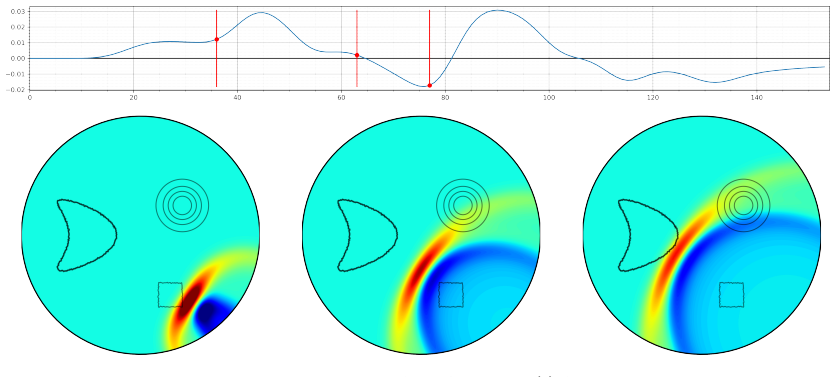
The load-bearing identity is (2.3), $I_{i,j}(t)=-\eta\int_\Omega p_j(x,t)H_i(x)\,dx$, which turns boundary voltage differences into weighted integrals of the interior power density $H_i=\sigma|\nabla u_i|^2$ against known acoustic fields. Step 1 expands $H_i$ in Neumann eigenfunctions (Bessel functions on the disk) and solves the resulting ill-conditioned system $\eta K\hat H_i=I_i$ with a smoothness penalty. Step 2 minimizes $J(\sigma)=\sum_i\|H_i(\sigma)-z_i\|_{L^1}+\beta|\sigma|_{TV}$ by iteratively reweighted quadratic subproblems. The ratio $\eta/\delta$ controls feasibility because the measured power signal is $O(\eta)$ while electrical noise is independent of $\eta$.
What would settle it
Use the same two-step algorithm on synthetic data where the pressure field used for inversion differs from the true field by a few percent in amplitude or timing, or where $\eta$ varies spatially; if the main phantom inclusions disappear at error levels consistent with clinical ultrasound, the feasibility claim as stated would fail.
Extended reading notes
Core claim
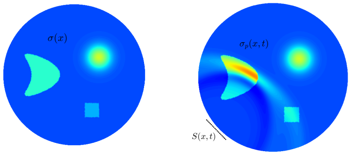
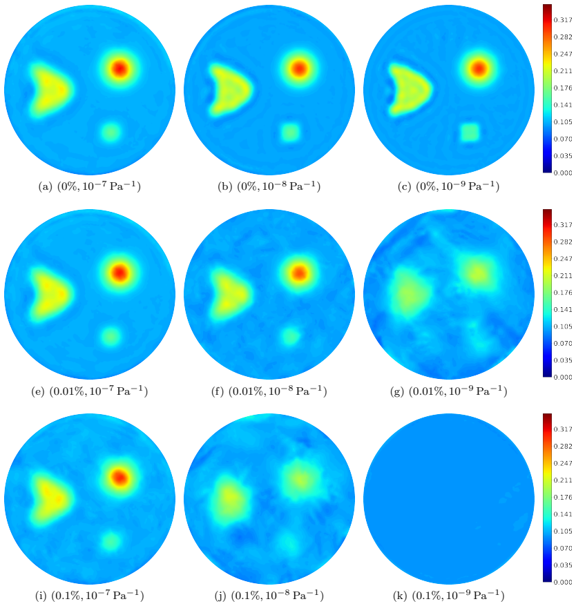
The paper reports that a complete two-step inversion pipeline for acousto-electric tomography can reconstruct interior conductivity from boundary measurements under realistic parameter choices. On the authors' terms: with the perturbed conductivity model $\sigma_p=\sigma(1+\eta p)$, the boundary power difference $I(t)$ is proportional to $\int p H\,dx$; collecting many acoustic source positions and boundary currents gives a linear system whose regularized solution yields the power density $H$. A second, total-variation-regularized optimization recovers $\sigma$ from $H$. In simulated experiments with 27 acoustic fields, 3 boundary currents, and noise up to $0.1\%$, the main features of high- and low-contrast phantoms are recovered for $\eta$ from $10^{-7}$ to $10^{-9}\,\mathrm{Pa}^{-1}$; at the smallest $\eta$ with $0.1\%$ noise the inclusions are barely visible. Limited-angle measurements reconstruct conductivity well near the measurement boundary, matching earlier observations.
Load-bearing premise
The whole pipeline assumes the acoustic pressure inside the body and the coupling constant $\eta$ are known exactly; if either is uncertain, the boundary time series cannot be converted into power density.
Editorial extensions
If this is right
- For the high-contrast phantom, the main inclusions are recovered for $\eta$ down to $10^{-8}\,\mathrm{Pa}^{-1}$ with up to $0.01\%$ noise; at $0.1\%$ noise the small square inclusion is nearly lost.
- Lower noise can compensate for smaller coupling: reconstructions at $\eta=10^{-8}$, $\delta=0.1\%$ and at $\eta=10^{-9}$, $\delta=0.01\%$ look similar, matching the predicted $\eta/\delta$ scaling.
- At zero noise, smaller $\eta$ improves reconstruction quality because the first-order linearization behind (2.3) becomes more accurate.
- With limited boundary access, inclusions close to the measurement boundary are recovered well, while deeper inclusions appear with reduced amplitude.
- Step 1 requires regularization; the singular values of the discretized operator decay exponentially, so unregularized least squares is not a viable route.
Reading between the lines
- A natural stress test is to add realistic uncertainty to the acoustic field itself, such as transducer position, timing, or wave-speed errors; the paper's stated idealization suggests this will degrade the first step, but how quickly is an open quantitative question.
- If $\eta$ varies by tissue type, the $\eta/\delta$ control suggests reconstructions will be locally feasible wherever $\eta/\delta$ is large, producing spatially varying contrast-to-noise rather than global success or failure.
- The two-step architecture could be used with other regularized linear solvers for step 1 and other data fidelities for step 2; the structural claim is the separation of the inversion into a linear ill-posed step and a nonlinear well-posed step.
Signed reviews
Editorial analysis
A structured set of objections, weighed in public.
Referee Report
Summary. The manuscript proposes a complete two-step computational inversion framework for acousto-electric tomography (AET). In Step 1, the interior power density H is reconstructed from boundary voltage time series by solving the linear Fredholm system (2.3), discretized with Neumann eigenfunctions and regularized by a Sobolev-type penalty (2.12). In Step 2, the conductivity sigma is recovered from H by minimizing the L1-TV functional (2.13) via an iteratively reweighted linearization (2.14). The authors perform synthetic numerical experiments with physically motivated parameters (eta between 10^-9 and 10^-7 Pa^-1, noise levels between 0% and 0.1%) and report that AET is feasible for medical imaging, including a limited-angle setup. The paper also derives the boundary-to-power-density identity (2.1) and discusses the dependence of reconstruction quality on the ratio eta/delta.
Significance. If the feasibility claim holds, this is a valuable contribution: it is one of the few studies that deliberately models both steps of AET and examines the eta/delta tradeoff in a realistic parameter regime. The derivation of the boundary-to-power-density identity (2.1) is clean, and the numerical experiments are internally consistent. However, the study's strength is conditional: the forward and inverse models share the same exact acoustic fields and the same constant eta, and the Step-1 regularization parameter is selected with oracle knowledge of the true solution. These idealizations bear directly on the feasibility claim. The paper explicitly acknowledges them in the conclusion, but they are not tested or mitigated. The manuscript would be strengthened by quantitative error assessment and by experiments that perturb the acoustic field and the coupling parameter.
major comments (4)
- [Section 2.1, Eqs. (2.3), (2.7), (2.11)] The first step assumes exact knowledge of the interior acoustic pressure field p_j(x,t_k) and the constant acousto-electric coupling eta. The kernel w^k_{j,n} in (2.7) and the linear system (2.11) require p_j as input, and the interpretation of I_{i,j} in (2.3) requires eta. The paper's own conclusion identifies 'accurate knowledge of the internal pressure field' as an idealization and notes that the assumption that eta is a known constant 'seems to be impractical.' Because the matrix K has exponentially decaying singular values (Fig. 4), errors in p_j or in eta will be amplified before regularization. The noise study in Section 3.2 perturbs only the boundary data g^k_{i,j}; it never perturbs p_j or eta. Thus the demonstrated eta/delta tradeoff may not transfer to a real instrument, and the central feasibility claim is not yet established under realistic uncertainty in the acoustic field.
- [Section 4.1, Eq. (2.12)] The regularization parameter beta in (2.12) is chosen 'optimally by computing the regularization-error curve and picking the minimum error choice,' i.e., using the true power density H. This is an oracle selection that provides an upper bound on achievable quality. A practical feasibility study should test a data-driven selection rule (e.g., Morozov discrepancy principle or an L-curve criterion) or at least report sensitivity of the reconstructions to beta. Without this, the reported quality of Step 1, and hence Step 2, is likely optimistic.
- [Section 1, Eq. (1.3) and Section 3.1] The assumption that eta is a known constant across the domain is inconsistent with the cited experimental values (eta about 4.1e-8 Pa^-1 in rabbit heart versus about 1e-9 Pa^-1 in saline), which suggest that eta is tissue-dependent. If eta varies spatially, the first-step equation (2.3) becomes I_{i,j}(t) = - Integral p_j(x,t) eta(x) H_i(x) dx, so the product eta H_i is what can be recovered, and separating eta from H would require additional information. The paper does not address this case, and the conclusion mentions it only in passing. This is a load-bearing gap for the claim of feasibility for medical imaging applications.
- [Section 4.2, Figs. 6-8] The conductivity reconstructions are assessed only visually; no quantitative error measures (e.g., relative L2 error, structural similarity, or contrast metrics) are reported. The central claim that the conductivity is 'well reconstructed' and the observed diagonal eta/delta pattern are supported only by qualitative inspection. Given that the paper's goal is to establish feasibility, quantitative assessment of the reconstructions is needed to substantiate the claim.
minor comments (5)
- [Section 2.1, Eq. (2.9)] The definition of the vector I_i is inconsistent: the last entry is written as I^{Nt}_{Nf,NS}, but since i is fixed, it should be I^{Nt}_{i,NS}, and the vector should lie in R^{NS Nt} rather than R^{Nf NS Nt} as printed.
- [Section 2.1, Eq. (2.12)] The expression 'hat H_i = min_{hat H in R^{N_phi}} ...' should read 'argmin' (or 'hat H_i = argmin'), since the right-hand side is a number and the left-hand side is a vector.
- [Table 1] The table caption contains a typo: 'Tabel' should be 'Table'.
- [Section 3.2] It would be helpful to state explicitly that the noise model does not perturb the acoustic field p or the coupling constant eta, since this is central to the interpretation of the numerical results.
- [Section 5 and Abstract] The abstract's statement that 'AET is indeed feasible for interesting applications' is stronger than what the experiments can support given the acknowledged idealizations; a more guarded phrasing would reflect the conditional nature of the results.
Circularity Check
No significant circularity: the two-step inversion is a self-contained numerical feasibility study whose idealizations are explicitly stated, not hidden inputs.
full rationale
The paper's derivation chain is not circular in the sense prohibited here. The forward model (2.1) produces boundary time series I from a known conductivity σ and acoustic field p; the inversion then recovers H by solving ηKĤ = I with kernel K built from the same p (2.7, 2.10, 2.11), and finally recovers σ from H via the TV-regularized problem (2.13). Data generation and inversion use the same acoustic fields, but this is a standard synthetic self-consistency test, not an equation reducing to its own input: the reconstructed σ is not the σ that generated the data by construction—it is the output of a regularized least-squares solve, and the paper reports noise-dependent degradation of quality. The assumptions that p and η are known are explicitly labeled idealizations in the conclusions, and the paper identifies them as such rather than presenting them as predictions. The regularization parameter β is chosen by an oracle ('picking the minimum error choice') to ensure comparability of reconstruction quality; while this is an optimistic methodological choice, it is not a fitted parameter renamed as a prediction. The limited-angle finding is corroborated by observation, not by self-citation alone. Self-citations to [1] and [21] are to computational methods and a prior observation; they are not load-bearing uniqueness theorems. No step exhibits the pattern of a fitted parameter being called a prediction or a definition being equivalent to its output. The skeptical concern about unmodeled acoustic-field uncertainty is a real limitation and is explicitly acknowledged by the authors, which further confirms it is not hidden or circularly resolved.
Assumptions & free parameters
free parameters (2)
- Step-1 regularization parameter beta in (2.12) =
not reported; chosen per experiment as the minimizer of true reconstruction error
- Step-2 TV regularization weight beta in (2.13) =
not reported
assumptions (4)
- domain assumption Acousto-electric coupling model sigma_p = sigma(1 + eta p) in (1.3) is exact and linear.
- domain assumption The first-order approximation u_p approximately u in (2.2) is accurate.
- domain assumption The acoustic pressure field p_j and coupling constant eta are known exactly.
- domain assumption Boundary measurements are continuous current and voltage on the whole boundary, not discrete electrodes.
Cite this review
Pith. "Pith review of Feasibility of Acousto-Electric Tomography." pith.science (2026). https://pith.science/paper/OSMUOBCD
@misc{pith2026190804215,
  author       = {Pith},
  title        = {Pith review of: Feasibility of Acousto-Electric Tomography},
  year         = {2026},
  howpublished = {\url{https://pith.science/paper/OSMUOBCD}},
  note         = {Machine review of arXiv:1908.04215}
}
read the original abstract
In acousto-electric tomography the goal is to reconstruct the electric conductivity in a domain from electrostatic boundary measurements of corresponding currents and voltages, while the domain is penetrated by a time-dependent acoustic wave. We explicitly model the phenomena, and we propose a complete inversion framework for acousto-electric tomography in two steps: First the interior power density is obtained from boundary measurements by solving a linear, ill-posed problem; second the interior conductivity is reconstructed from the power density by solving a non-linear, fairly well-posed problem. We perform numerical experiments on synthetic data with realistically chosen parameters. We investigate how feasibility of reconstructing the electrical conductivity from boundary measurements depends on the acousto-electric coupling constant and measurement noise. Our findings are positive, and indicate that AET is indeed feasible for interesting applications in for example medical imaging. Finally, we consider a limited angle setup and show that the conductivity is well reconstructed near the measurement boundary.
Figures

Figures from the paper (5 more)



Reference graph
Works this paper leans on
-
[1]
B. J. Adesokan, B. Jensen, B. Jin, and K. Knudsen. Acousto-electric tomography with total variation regularization. Inverse Problems, 35(3):035008, 25, 2019
work page 2019
-
[2]
B. J. Adesokan, K. Knudsen, V. P. Krishnan, and S. Roy. A fully non-linear optimization approach to acousto-electric tomography. Inverse Problems, 34(10):104004, 2018. 13 (a) (0%, 10−7 Pa−1) (b) (0%, 10−8 Pa−1) (c) (0%, 10−9 Pa−1) (e) (0.01%, 10−7 Pa−1) (f) (0.01%, 10−8 Pa−1) (g) (0.01%, 10−9 Pa−1) (i) (0.1%, 10−7 Pa−1) (j) (0.1%, 10−8 Pa−1) (k) (0.1%, 10...
work page 2018
-
[3]
G. S. Alberti and Y. Capdeboscq. Lectures on elliptic methods for hybrid inverse problems , volume 25. Soci´ et´ e Math´ ematique de France, 2018
work page 2018
- [4]
-
[5]
G. Bal, C. Guo, and F. Monard. Imaging of anisotropic conductivities from current den- sities in two dimensions. SIAM J. Imaging Sci. , 7(4):2538–2557, 2014
work page 2014
-
[6]
G. Bal, K. Hoffmann, and K. Knudsen. Propagation of singularities for linearised hybrid data impedance tomography. Inverse Problems, 34(2):024001, 19, 2018. 14 (a) (0%, 10−8 Pa−1) (b) (0.01%, 10−8 Pa−1) (c) (0.1%, 10−8 Pa−1) Figure 8: Mixed high contrast phantom reconstructions with limited boundary measurements. Each is marked with its corresponding ( δ,η...
work page 2018
-
[7]
G. Bal, W. Naetar, O. Scherzer, and J. Schotland. The Levenberg-Marquardt iteration for numerical inversion of the power density operator. J. Inverse Ill-Posed Probl. , 21(2):265– 280, 2013
work page 2013
-
[8]
D. C. Barber and B. H. Brown. Applied potential tomography. Journal of Physics E: Scientific Instruments, 17(9):723, 1984
work page 1984
Show all 37 references
-
[9]
H. K. Bidhendi, H. M. Jafari, and R. Genov. Ultra-wideband imaging systems for breast cancer detection. In Ultra-Wideband and 60 GHz Communications for Biomedical Appli- cations, pages 83–103. Springer, 2014
2014
-
[10]
Capdeboscq, J
Y. Capdeboscq, J. Fehrenbach, F. de Gournay, and O. Kavian. Imaging by modifica- tion: Numerical reconstruction of local conductivities from corresponding power density measurements. SIAM Journal on Imaging Sciences , 2(4):1003–1030, 2009
2009
-
[11]
Cheney, D
M. Cheney, D. Isaacson, and J. C. Newell. Electrical impedance tomography. Siam Review, 41(1):85–101, 1999
1999
-
[12]
Cherepenin, A
V. Cherepenin, A. Karpov, A. Korjenevsky, V. Kornienko, A. Mazaletskaya, D. Mazourov, and D. Meister. A 3D electrical impedance tomography (EIT) system for breast cancer detection. Physiological measurement, 22(1):9, 2001
2001
-
[13]
M. Demi. 2.12 - the basics of ultrasound. In A. Brahme, editor, Comprehensive Biomedical Physics, pages 297 – 322. Elsevier, Oxford, 2014
2014
-
[14]
L. C. Evans. Partial differential equations. American Mathematical Society,, 2010
2010
-
[15]
Fabrizi, A
L. Fabrizi, A. Mcewan, E. J. Woo, and D. Holder. Analysis of resting noise characteristics of three eit systems in order to compare suitability for time difference imaging with scalp electrodes during epileptic seizures. Physiological measurement, 28:S217–36, 08 2007
2007
-
[16]
Gebauer and O
B. Gebauer and O. Scherzer. Impedance-acoustic tomography. SIAM J. Appl. Math. , 69(2):565–576, 2008
2008
-
[17]
P. C. Hansen. Discrete inverse problems: insight and algorithms , volume 7. Siam, 2010
2010
-
[18]
S. M. Hesabgar, A. Sadeghi-Naini, G. Czarnota, and A. Samani. Dielectric properties of the normal and malignant breast tissues in xenograft mice at low frequencies (100 hz–1 mhz). Measurement, 105:56–65, 2017. 15
2017
-
[19]
Hoffmann and K
K. Hoffmann and K. Knudsen. Iterative reconstruction methods for hybrid inverse problems in impedance tomography. Sens. Imaging, 15(1):art. id. 96, 2014
2014
-
[20]
D. S. Holder. Electrical Impedance Tomography: Methods History and Applications, Series in Medical Physics and Biomedical Engineering . IOP Press,, 2010
2010
-
[21]
Hubmer, K
S. Hubmer, K. Knudsen, C. Li, and E. Sherina. Limited-angle acousto-electrical tomogra- phy. Inverse Problems in Science and Engineering , 27(9):1–20, 2018
2018
-
[22]
W. T. Joines, Y. Zhang, C. Li, and R. L. Jirtle. The measured electrical properties of normal and malignant human tissues from 50 to 900 mhz. Medical physics, 21(4):547–550, 1994
1994
-
[23]
Kress, V
R. Kress, V. Maz’ya, and V. Kozlov. Linear integral equations, volume 82. Springer, 1989
1989
-
[24]
Kuchment and L
P. Kuchment and L. Kunyansky. Synthetic focusing in ultrasound modulated tomography. Inverse Problems and Imaging , 4(4):665–673, 2010
2010
-
[25]
Kuchment and L
P. Kuchment and L. Kunyansky. 2D and 3D reconstructions in acousto-electric tomography. Inverse Problems, 27(5):055013, 2011
2011
-
[26]
Q. Li, R. Olafsson, P. Ingram, Z. Wang, and R. Witte. Measuring the acoustoelectric interaction constant using ultrasound current source density imaging. Physics in Medicine & Biology, 57(19):5929, 2012
2012
-
[27]
Logg, K.-A
A. Logg, K.-A. Mardal, and G. Wells. Automated solution of differential equations by the finite element method: The FEniCS book , volume 84. Springer Science & Business Media, 2012
2012
-
[28]
M. M. Mellenthin, J. L. Mueller, E. D. L. B. de Camargo, F. S. de Moura, T. B. R. Santos, R. G. Lima, S. J. Hamilton, P. A. Muller, and M. Alsaker. The ace1 electrical impedance tomography system for thoracic imaging. IEEE Transactions on Instrumentation and Measurement, 2018
2018
-
[29]
Monard and D
F. Monard and D. Rim. Imaging of isotropic and anisotropic conductivities from power densities in three dimensions. Inverse Problems, 34(7):075005, 26pp, 2018
2018
-
[30]
Roy and A
S. Roy and A. Borz` ı. A new optimization approach to sparse reconstruction of log- conductivity in acousto-electric tomography.SIAM J. Imaging Sci., 11(2):1759–1784, 2018
2018
-
[31]
Y. Saad. Numerical methods for large eigenvalue problems: revised edition , volume 66. Siam, 2011
2011
-
[32]
Somersalo, M
E. Somersalo, M. Cheney, and D. Isaacson. Existence and uniqueness for electrode mod- els for electric current computed tomography. Siam Journal on Applied Mathematics , 52(4):1023–1040, 1992
1992
-
[33]
X. Song, Y. Xu, and F. Dong. An image reconstruction framework based on boundary voltages for ultrasound modulated electrical impedance tomography. Measurement Science and Technology, 27(11):114003, 2016
2016
-
[34]
W. A. Strauss. Partial differential equations: An introduction . Wiley, 2007
2007
-
[35]
B. E. Treeby and B. T. Cox. k-wave: Matlab toolbox for the simulation and reconstruction of photoacoustic wave fields. Journal of biomedical optics , 15(2):021314, 2010
2010
-
[36]
Widlak and O
T. Widlak and O. Scherzer. Hybrid tomography for conductivity imaging. Inverse Prob- lems, 28(8):084008, 28, 2012. 16
2012
-
[37]
Zhang and L
H. Zhang and L. V. Wang. Acousto-electric tomography. Progress in Biomedical Optics and Imaging - Proceedings of Spie , 5(9):20, 145–149, 2004. 17
2004
Reviewed August 14, 2026 · model on record in the stance chip above.
Discussion (0). Continue with ORCID to comment.