A Pseudospectral Method for the One-Dimensional Fractional Laplacian on $\mathbb R$

Carlota M. Cuesta; Francisco de la Hoz; Jorge Cayama

REVIEW 3 major objections 6 minor 47 references

A Pseudospectral Method for the One-Dimensional Fractional Laplacian on $\mathbb R$

T0 review · 3 major / 6 minor · reviewed 2026-08-14 · deepseek-v4-flash

Challenge this review Re-run · record.json Download PDF Read on arXiv ↗ Review JSON

Pith's one-line read This paper establishes explicit Fourier series formulas for the fractional Laplacian of trigonometric modes on the whole real line, packaged as an operational matrix.

desk verdict Genuinely new explicit formulas for the fractional Laplacian of Fourier modes, with strong numerical tests, but the spectral accuracy claim is only as good as the smoothness of the periodic extension of the mapped function, and the paper never tests a case where that extension is not flat at the endpoints. read the letter →

arxiv 1908.09143 v1 pith:OXVPVX2M submitted 2019-08-24 math.NA cs.NA

Jorge Cayama , Carlota M. Cuesta , Francisco de la Hoz This is my paper · ORCID

classification math.NAcs.NA MSC 65M7035R1165T50

keywords fractionalLaplacianpseudospectralmethodsrationalChebyshevfunctionsFourierseriesnonlocalFisherequationoperationalmatrixwhole-linecomputation

verification ladder T0 review T1 audit T2 compute T3 formal

The pith

A machine-rendered reading of the paper's core claim, the machinery that carries it, and where it could break.

The reading

The paper aims to compute $(-\Delta)^{\alpha/2}u$ numerically for smooth bounded functions on the whole real line, without truncating the domain to a finite interval. It maps $x\in\mathbb R$ to $s\in[0,\pi]$ via $x=L\cot(s)$, expands the mapped function as a finite Fourier series, and reduces the whole task to the action of the fractional Laplacian on one mode $e^{iks}$. The central result is an explicit infinite-series formula for $(-\Delta)^{\alpha/2}e^{iks}$, encoded in an operational matrix. If the formula is correct, a user can approximate the fractional Laplacian for any regular function at spectral accuracy using only three choices: the mode count $N$, a truncation level $l_{\rm lim}$, and the scale $L$. The authors test the method on explicit examples and use it to simulate Fisher's equation with fractional diffusion in the monostable case, recovering the theoretically predicted exponentially accelerating front speed.

What carries the argument

The machinery is the composition of three steps. First, Lemma 2.1 rewrites the singular integral definition (1) as a Hilbert transform when $\alpha=1$ and as a second-derivative integral kernel $\frac{c_\alpha}{\alpha(1-\alpha)}\int u_{xx}(y)|x-y|^{\alpha-1}\,dy$ otherwise, requiring only bounded $C^2$ functions. Second, the algebraic map $x=L\cot(s)$ turns $\mathbb R$ into the finite interval $[0,\pi]$ and Chebyshev or rational-Chebyshev series into Fourier series, so the operator acts on modes $e^{iks}$. Third, Theorem 2.2 supplies the explicit action on each mode, and Section 2.5 packages it as an operational matrix $M_\alpha$ evaluated on the pseudospectral nodes $s_j=\pi(2j+1)/(2N)$, with the infinite $l$-sum folded by aliasing into $l_1,l_2$ blocks and stabilized Gamma-function ratios computed recursively.

What would settle it

Recompute the integrals $I_1$ and $I_2$ in (24) by an independent method, such as residue calculus or high-precision quadrature of the original singular integral (13) for a moderately odd $k$ and a few values of $\alpha$, and compare with (18); a discrepancy at the level of machine precision in the odd-$k$ branch, where no closed form is available for comparison, would falsify the central formula.

Watch

Extended reading notes

Core claim

The paper's central discovery is Theorem 2.2: for $\alpha\in(0,1)\cup(1,2)$, the fractional Laplacian of the elementary trigonometric function $e^{iks}$ on $\mathbb R$, after the mapping $x=L\cot(s)$, equals an infinite series over $l\in\mathbb Z$ (equation (18), with separate even-$k$ and odd-$k$ branches), and for $\alpha=1$ the same object is given by equation (19). The coefficients are ratios of Gamma functions with absolute-value arguments, multiplied by factors involving $\cot(\pi\alpha/2)$ or a sign factor. This formula is the load-bearing component: once it is known, the fractional Laplacian of a Fourier-expanded function is obtained by applying the corresponding matrix $M_\alpha$ to the Fourier coefficients, with no domain truncation anywhere.

Load-bearing premise

The method rests on the computer-algebra evaluation of the integrals $I_1$ and $I_2$ in (24), which the text reports without an independent derivation, together with an unstated periodicity of $|\sin(s-\eta)|^{\alpha-1}$; if either ingredient is wrong, Theorem 2.2 and the matrix $M_\alpha$ collapse.

Editorial extensions

If this is right

For any bounded regular function approximated by its $2N$-point Fourier interpolant (15), the fractional Laplacian at the nodes is approximated by a matrix-vector product; tests on $e^{i2s}$ and $e^{-x^2}$ show errors below $10^{-12}$ for large enough $N$ and $l_{\rm lim}$.
The method avoids truncation error entirely because the map covers all of $\mathbb R$; the only controlled parameters are $N$, $l_{\rm lim}$, and the map scale $L$, with $L$ tunable by spectral interpolation without recomputing the matrix from scratch.
For even $k$ the formula reproduces known closed forms (e.g. (37) for $k=2$ and the Gaussian formula (39)); for odd $k$ it provides the first explicit series representation, with a special treatment at $\alpha=1$.
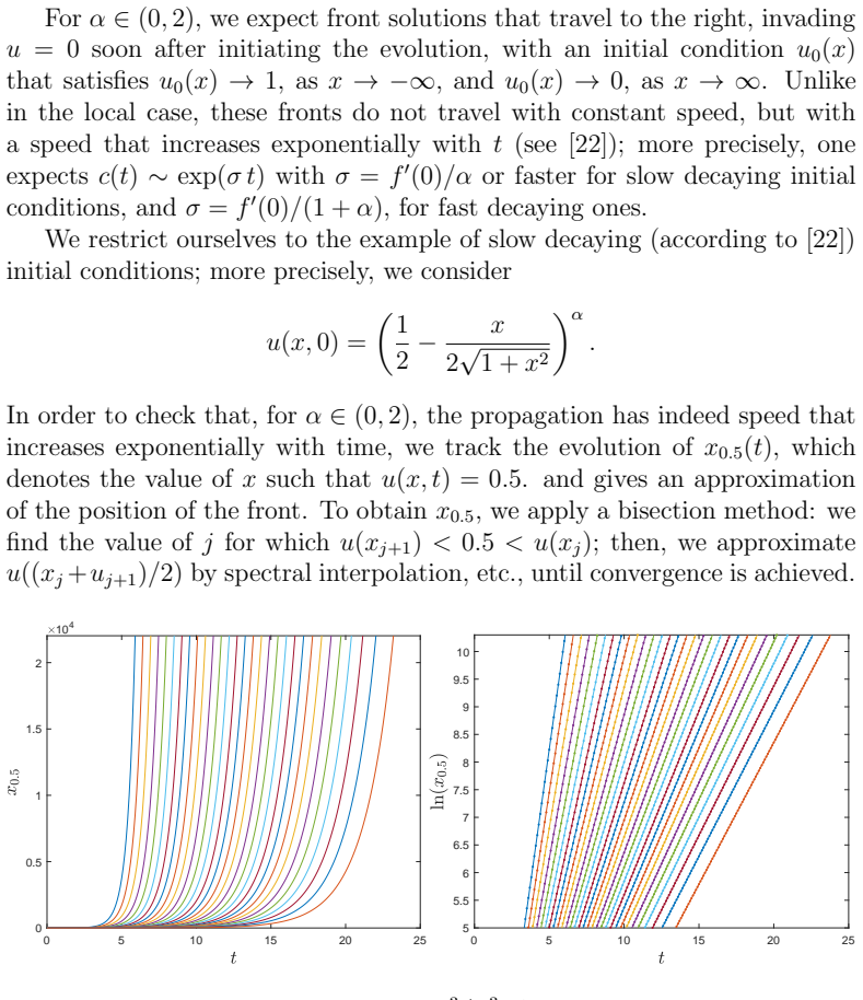
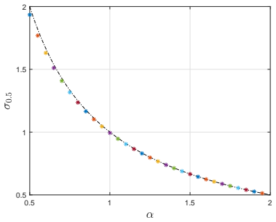
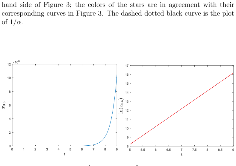
The Fisher-KPP simulation confirms the theoretical prediction $c(t)\sim e^{t/\alpha}$ for monostable fractional fronts; the measured slope $\sigma_{0.5}$ approaches $1/\alpha$ as $\alpha\to2^-$, and for $\alpha=0.5$ increases to $1.9865$ when $N$ and $L$ are enlarged.

Reading between the lines

Editorial extensions of the paper, not claims the author makes directly.

If Theorem 2.2 holds, the same mode-by-mode strategy should extend to other kernels that are diagonalized by the cotangent map, such as Riesz derivatives or Hilbert-type operators, and even to $L^2(\mathbb R)$ functions whose mapped versions have converging Fourier series.
Because the Hilbert transform is diagonalized by the sine-like basis functions mentioned in the paper, the odd-$k$ formula at $\alpha=1$ could be checked directly against that basis, a computation the paper does not perform.
A testable practical extension would be an automatic rule for choosing $l_{\rm lim}$ and $L$ as functions of $\alpha$, $N$, and the decay of the target function; the paper gives heuristics but no selection criterion.

Share X Bluesky LinkedIn Reddit HN

Signed reviews

No signed human review yet.

Editorial analysis

A structured set of objections, weighed in public.

Desk editor's note, referee report, and a circularity audit.

Desk Editor's Note

read the letter

Two things to know. First, the explicit computation of (-Delta)^{alpha/2}e^{iks} in Theorem 2.2 is a real addition to the spectral toolbox for fractional operators on R; the x = L cot(s) mapping plus aliasing-aware truncation is a coherent way to avoid domain truncation. Second, the paper's claim about arbitrary bounded regular functions is broader than what is actually shown: the pseudospectral coefficients are those of a 2pi-periodic extension of u(L cot s), and the convergence rate is controlled by the smoothness of that extension, not just by the smoothness of u on R.

The paper does several things well. The operational matrix construction is thoughtful, especially the recursive gamma-function ratios and the l = l1 N + l2 aliasing decomposition. The numerical validation is genuinely strong: the e^{i2s} test reaches 5e-13 and the Gaussian test reaches 1e-12 against an independent exact formula, over a wide sweep of alpha. The Fisher front simulation matching the predicted exp(t/alpha) growth is also credible evidence that the method works in a nontrivial time-dependent setting.

I am less worried than the reader's report about the Mathematica step. The proof of Theorem 2.2 does delegate the key integrals I1 and I2 to a CAS without derivation, and that should be fixed. But the Gaussian benchmark independently checks the resulting even- and odd-mode formulas across many alpha values, so the CAS result is empirically corroborated. That is not nothing.

The weakest point is the one the stress-test note identifies: the extension. For u(x) = arctan(x), the mapped function u(L cot s) has first-derivative jumps at s = 0 and s = pi after the standard even extension, so the Fourier coefficients decay only as O(k^{-2}) and the method reduces to algebraic, not spectral, accuracy. The paper tests only functions whose mapped versions are either periodic or flat at both endpoints, so the abstract's blanket claim for any bounded regular function is unsupported. There is also no convergence analysis, no code, and the ad hoc setting of the e^{-iNs} mode to zero deserves justification, though that is a minor concern in practice.

This paper deserves a serious referee. I would send it for review and ask for a revision: prove or at least derive the CAS integrals, test a function with unequal limits at plus and minus infinity, and either weaken the abstract's generality or explain the extension smoothness condition.

Referee Report

3 major / 6 minor

Summary. The paper proposes a pseudospectral method for computing the one-dimensional fractional Laplacian on R without truncating the domain. The authors map x to s via x = L cot(s), represent a function u(x) as a Fourier series in s, and derive in Theorem 2.2 explicit infinite-series formulas for (-Delta)^{alpha/2} e^{iks}. These formulas are used to build a differentiation matrix M_alpha acting on Fourier coefficients. Numerical tests compare the method against exact expressions for e^{i2s} and exp(-x^2), and the method is applied to Fisher-KPP fronts to recover the predicted exponential acceleration e^{t/alpha}. The paper claims that the method approximates the fractional Laplacian accurately and efficiently for bounded regular functions without truncation.

Significance. If Theorem 2.2 is correct, the operational-matrix construction is elegant and potentially useful: the matrix is reusable, the gamma-function factorization in (32)-(33) gives a stable implementation, and the benchmark results are quantitatively strong (errors near 1e-12 for e^{i2s}, 8e-12 for exp(-x^2), and Fisher slope estimates close to 1/alpha). The Gaussian test against the independent formula (39) and the Fisher front comparison with the Cabre-Roquejoffre theory provide genuine external validation. However, the paper's stated scope is broader than what is proved: the central derivation relies on unverified computer-algebra evaluations, no convergence or tail estimates are given for the series and matrix truncations, and the Fourier-extension step is not analyzed for general bounded C^infty functions with different limits at +/-infinity. With these gaps addressed, the paper would be a useful contribution to spectral methods for fractional operators.

major comments (3)

[Theorem 2.2, Eqs. (24)-(30)] The proof of the central formulas delegates the evaluation of I1 and I2 to Mathematica without an independent derivation. Since every subsequent formula and the matrix M_alpha rest on these evaluations, a complete derivation or a reproducible computer-algebra script is needed; the empirical benchmark against (39) is good evidence but does not replace a proof. In addition, the factorization d_kl = (1/pi) I1 I2 in Eq. (24) silently uses the pi-periodicity of |sin(s-eta)|^{alpha-1} and of e^{-i2ls} to shift the inner integration interval, which produces the factor e^{-i2l eta} that turns e^{ik eta} into e^{i(k-2l) eta}; this step should be stated explicitly.
[Section 2.3 and Section 3] The accuracy of representation (15) is governed by the smoothness of the even extension of u(s) to [0,2pi], not by the smoothness of u(x). For u(x) = arctan x with L = 1, u(s) = arctan(cot s) satisfies u_s(pi^-) = -1, while the even extension has u_s(pi^+) = +1, so the first derivative jumps and the Fourier coefficients decay only as O(k^{-2}); the L_infinity truncation error is then O(N^{-1}), not spectral. The tests in Section 3 use only finite Fourier modes and exp(-x^2), whose mapped version is flat at s = 0 and s = pi, so the abstract's claim for arbitrary bounded regular functions is unsupported. Please either prove an error estimate for the extension or explicitly restrict the class of functions considered.
[Section 2.5, around Eq. (31)] The assignment (-Delta)^{alpha/2}(e^{-iNs}) = 0 is introduced because \hat u(-N) = \hat u(N), and the truncation of the l-sum at l_lim is justified only by numerical stability. Both choices inject uncontrolled errors into M_alpha, and the abstract's phrase 'without using truncation' is misleading because the method truncates the Fourier series, the l-sum, and applies a Krasny filter. Please provide tail estimates for the l-sum and an error bound for the highest-mode treatment, or state these as heuristic parameters in a clearly delimited claim.

minor comments (6)

[Eq. (19)] In the second case of Eq. (19), the series over l includes l = 0, where sgn(l) is undefined; please specify that the l = 0 term is the separate constant -2/(k^2-4) and that the series runs over l != 0.
[Section 4, paragraph after Eq. (41)] The bisection description contains a typo: 'u((x_j + u_{j+1})/2)' should read 'u((x_j + x_{j+1})/2)'.
[Figure 2 caption] The caption says L in {0.1, 0.2, ..., 1}, while the text says L in {0.1, 0.2, ..., 10}; one of these is wrong.
[References] Reference [28] is incomplete: it lacks volume, year, and page numbers.
[Eq. (37)] The expression (-i sin(s) e^{is})^{1+alpha} requires a branch choice; please state the principal branch used in the numerical comparisons.
[Section 2.3] The phrase 'spacial shift' should be 'spatial shift'.

Circularity Check

0 steps flagged · score 0.0 of 10

No significant circularity: the central formulas are derived from first principles (with CAS-assisted integrals) and benchmarked against independent external results; self-citations are methodological only.

full rationale

The paper's load-bearing result is Theorem 2.2, an explicit formula for (-Δ)^{α/2} e^{iks} obtained by substituting u=e^{iks} into the mapped integral representation (13) and evaluating the coefficient integrals I1 and I2. The evaluation is delegated to Mathematica, but the theorem is not assumed; it is computed from the stated representation. The numerical method then applies this formula to the Fourier coefficients of u(s) via the matrix M_α in (31). No parameter is fitted to any target output: N, l_lim, and L are user-chosen discretization parameters. The tests do not secretly reproduce the inputs. Table 1 compares the implemented formula (34) with the closed form (37) for e^{i2s}; both expressions come from the same integral representation and are obtained with Mathematica, so this is an internal consistency check rather than an external benchmark, but it is not circular because (37) is a separate symbolic evaluation that the series formula must reduce to, not a fitted value. The Gaussian example uses the independent formula (39) from Pozrikidis [4], and the Fisher-front slopes are compared with the Cabré–Roquejoffre prediction e^{t/α}, an external analytical result. The self-citations ([23], [30]) are methodological: [23] suggests the cotangent mapping and the Fourier-mode operational-matrix idea, but the fractional-Laplacian calculation here is carried out in this paper rather than imported. There is no uniqueness theorem invoked from the authors' prior work and no ansatz smuggled in by citation. The main caveat noted in the manuscript, that non-smooth periodic extensions of u(s) limit Fourier decay, is a correctness/accuracy limitation, not circularity.

Assumptions & free parameters 3 free parameters · 5 assumptions · 0 invented entities

The central claim rests on three groups of assumptions: (i) the function regularity and decay conditions in Lemma 2.1; (ii) unproved CAS integral evaluations in Theorem 2.2; (iii) ad hoc numerical choices (mode e^{-iNs} set to zero, l_lim truncation, L selection). The method's correctness is empirically supported by the tests, but the derivation is not self-contained.

free parameters (3)

L = 1 in basic tests; 4.6 optimal for Gaussian with N=64; 1000/alpha^3 for Fisher simulations
Mapping scale in x = L cot(s). Accuracy depends strongly on L (Fig. 2). Chosen by hand or after trials, no rigorous optimal selection.
l_lim = up to 500 or N-dependent, e.g., 70 to 530
Truncation of the infinite series over l in (18)/(34). Chosen large enough to reach errors around 5e-13; no error estimate.
Krasny filter threshold = machine epsilon
Fourier coefficients below this threshold are set to zero; a standard spectral filter, but a user-chosen parameter.

assumptions (5)

domain assumption u is in C^2_b(R), and for alpha in (0,1) additionally lim_{x to +-infty} u_x(x) = 0.
Lemma 2.1 uses integration by parts representations requiring these smoothness and decay conditions; the method inherits them.
ad hoc to paper The integrals I1 and I2 in (25)-(29) are evaluated correctly by Mathematica.
The central theorem (18) depends on these CAS computations; no proof is given in the paper.
domain assumption The function u(s) admits a rapidly convergent Fourier series over s in [0,2pi] after a suitable extension (even or odd) at s = pi.
The pseudospectral approximation (15) and its accuracy rely on the smoothness of the extended function; the paper notes this is 'not a minor point'.
ad hoc to paper Aliasing in the series (18): l can be decomposed as l = l1 N + l2 and the l1 sum can be truncated at l_lim without significant error.
The numerical implementation (34)-(35) uses this truncation; no error bound is provided.
ad hoc to paper The highest mode e^{-iNs} is assigned zero fractional Laplacian.
Section 2.5 imposes (-Delta)^{alpha/2}(e^{-iNs}) = 0 to avoid the discrepancy between u-hat(-N) and u-hat(N); this is unjustified.

how reviews work

0 comments

Cite this review

Pith. "Pith review of A Pseudospectral Method for the One-Dimensional Fractional Laplacian on $\mathbb R$." pith.science (2026). https://pith.science/paper/OXVPVX2M

@misc{pith2026190809143,
  author       = {Pith},
  title        = {Pith review of: A Pseudospectral Method for the One-Dimensional Fractional Laplacian on $\mathbb R$},
  year         = {2026},
  howpublished = {\url{https://pith.science/paper/OXVPVX2M}},
  note         = {Machine review of arXiv:1908.09143}
}

abstract

In this paper, we propose a novel pseudospectral method to approximate accurately and efficiently the fractional Laplacian without using truncation. More precisely, given a bounded regular function defined over $\mathbb R$, we map the unbounded domain into a finite one, then we represent the function as a trigonometrical series. Therefore, the central point of this paper is the computation of the fractional Laplacian of an elementary trigonometric function. As an application of the method, we also do the simulation of Fisher's equation with fractional Laplacian in the monostable case.

Figures

Figures reproduced from arXiv: 1908.09143 by the authors.

**Figure 1.** Maximum global error for N = 128, as a function of llim. Let us consider now a function with Gaussian decay, u3 = exp(−x 2 ), such that (see, for instance, [4, pp. 29-30]). (−∆)α/2u3(x) = 2 αΓ(1/2 + α/2) √ π 1F1(1/2 + α/2, 1/2, −x 2 ), (39) where 1F1 is the Kummer confluent hypergeometric function, which can be evaluated accurately, among others, by Matlab (with the command hypergeom) and Mathematica (with the comma… view at source ↗

**Figure 2.** Maximum global error for N = 64, and L ∈ {0.1, 0.2, . . . , 1}, considering an even extension and an odd extension. Although there are some theoretical results [43], the optimal value of L depends on more than one factor: number of points, class of functions, type of problem, etc (see also [30, 23]). For instance, in the case of (−∆)α/2 , the best choice of L might depend on α, too. However, a good working rule of t… view at source ↗

**Figure 3.** α = 0.5, 0.55, . . . , 1.95, L = 103/α3 , ∆t = 0.01 and N = 1024. Left: x0.5(t) against t. Right: ln(x0.5(t)) against t, and the corresponding leastsquare fitting lines. In both subfigures, the curves are ordered according to α: the left-most ones correspond to α = 0.5, and the right-most ones, to α = 1.95. 24 [PITH_FULL_IMAGE:figures/full_fig_p024_3.png] view at source ↗

Figures from the paper (2 more)

**Figure 4.** Figure 4: Slopes of the least-square fitting lines, as obtained in the right [PITH_FULL_IMAGE:figures/full_fig_p026_4.png]

**Figure 5.** Figure 5: α = 0.5, L = 104 , ∆t = 5 · 10−3 , and N = 8192. Left: x0.5(t) against t ∈ [0, 9]. Right: ln(x0.5(t)) against t ∈ [5, 9], and the corresponding least-square fitting line. 26 [PITH_FULL_IMAGE:figures/full_fig_p026_5.png]

Discussion (0). Continue with ORCID to comment.

Reference graph

Works this paper leans on

47 extracted references · 45 canonical work pages

[1]

A. L. et al., What is the Fractional Laplacian?, arXiv:1801.09767v1 [math.NA]

arXiv
[2]

Kwa´ snicki, Ten equivalent deﬁnitions of the Fractional Laplace Op- erator, Fract

M. Kwa´ snicki, Ten equivalent deﬁnitions of the Fractional Laplace Op- erator, Fract. Calc. Appl. Anal. 20 (1) (2017) 7–51

work page 2017
[3]

Hilbert, Grundz¨ uge einer allgemeinen Theorie der linearen Integral- gleichungen, Fortschritte der Mathematischen Wissenschaften in Mono- graphien, Druck und Verlag von B

D. Hilbert, Grundz¨ uge einer allgemeinen Theorie der linearen Integral- gleichungen, Fortschritte der Mathematischen Wissenschaften in Mono- graphien, Druck und Verlag von B. G. Teubner, Leipzig und Berlin, 1912, in German

work page 1912
[4]

Pozrikidis, The Fractional Laplacian, CRC Press, Boca Raton, FL, 2016

C. Pozrikidis, The Fractional Laplacian, CRC Press, Boca Raton, FL, 2016

work page 2016
[5]

Kolmogorov, I

A. Kolmogorov, I. Petrovsky, N. Piscounov, Study of the Diﬀusion Equa- tion with Growth of the Quantity of Matter and its Application to a Biology Problem, Dynamics of Curved Fronts (1988) 105–130

work page 1988
[6]

R. A. Fisher, The wave of advance of advantageous genes, Annals of Eugenics 7 (1937) 355–369

work page 1937
[7]

A. M. Wazwaz, A. Gorguis, An analytic study of Fishers equation by using Adomian decomposition method, Applied Mathematics and Com- putation 154 (3) (2004) 609–620

work page 2004
[8]

V. G. Danilov, V. P. Maslov, K. A. Vosolov, Mathematical modelling of Heat and Mass Transfer Processes, Kluwer, Dordrecht, 1995

work page 1995

Show all 47 references

[9]

A. D. Polyanin, V. F. Zaitsev, Handbook of Nonlinear Partial Diﬀeren- tial equation, 1st Edition, Chapman and Hall/CRC press, 2003. 27

2003
[10]

C. F. Starmer, V. N. Biktashev, D. N. Romashko, M. R. Stephanov, O. N. Makarova, V. I. Krinsky, Vulnerability in excitable medium: An- alytical and numerical studies of initiating unidirectional propagation, Biophysical Journal 65 (5) (1993) 1775–1787

1993
[11]

J. P. Keener, J. Sneyd, Mathematical physiology, Vol. 1, Springer, New York, 1998

1998
[12]

FitzHugh., Impulses and Physiological States in Theoretical Models of Nerve Membrane, Biophysical Journal 1 (6) (1961) 445–466

R. FitzHugh., Impulses and Physiological States in Theoretical Models of Nerve Membrane, Biophysical Journal 1 (6) (1961) 445–466

1961
[13]

Nagumo, S

J. Nagumo, S. Arimoto, S. Yoshizawa, An Active Pulse Transmission Line Simulating Nerve Axon, Proceedings of the IRE 50 (10) (1962) 2061–2070

1962
[14]

C. E. F. Schl¨ ogl, R. S. Berry, Fluctuations in the interface between two phases, Physical Review A. 27 (5) (1983) 2698–2704

1983
[15]

Mancinelli, D

R. Mancinelli, D. Vergni, A. Vulpiani, Superfast front propagation in reactive systems with non-gaussian diﬀusion, Europhysics Letters 60 (4) (2002) 532–538

2002
[16]

Mancinelli, D

R. Mancinelli, D. Vergni, A. Vulpiani, Front propagation in reactive systems with anomalous diﬀusion, Physica D: Nonlinear Phenomena 185 (3–4) (2003) 175–195

2003
[17]

Baeumer, M

B. Baeumer, M. Kov´ acs, M. M. Meerschaert, Numerical solutions for fractional reaction-diﬀusion equations, Computers & Mathematics with Applications 55 (10) (2008) 2212–2226

2008
[18]

Cabr´ e, Y

X. Cabr´ e, Y. Sire, Nonlinear equations for fractional Laplacians, I: Reg- ularity, maximum principles, and Hamiltonian estimates, Annales de l’Institut Henri Poincar´ e. Analyse Non Lin´ eaire 31 (1) (2014) 23–53

2014
[19]

Cabr´ e, Y

X. Cabr´ e, Y. Sire, Nonlinear equations for fractional Laplacians II: Exis- tence, uniqueness, and qualitative properties of solutions, Transactions of the American Mathematical Society 367 (2) (2015) 911–941

2015
[20]

Engler, On the speed of spread for fractional reaction-diﬀusion equa- tions, International Journal of Diﬀerential Equations16 pages

H. Engler, On the speed of spread for fractional reaction-diﬀusion equa- tions, International Journal of Diﬀerential Equations16 pages. 28
[21]

Cabr´ e, J.-M

X. Cabr´ e, J.-M. Roquejoﬀre, Propagation de fronts dans les ´ equations de Fisher-KPP avec diﬀusion fractionnaire, Comptes Rendus Math´ ematique. Acad´ emie des Sciences. Paris 347 (23-24) (2009) 1361– 1366

2009
[22]

Cabr´ e, J.-M

X. Cabr´ e, J.-M. Roquejoﬀre, The inﬂuence of fractional diﬀusion in Fisher-KPP equations, Communications in Mathematical Physics 320 (3) (2013) 679–722

2013
[23]

de la Hoz, C

F. de la Hoz, C. M. Cuesta, A pseudo-spectral method for a non-local KdV-Burgers equation posed on R, Journal of Computational Physics 311 (2016) 45–61

2016
[24]

A. A. Kilbas, H. M. Srivastava, J. J. Trujillo, Theory and Applications of Fractional Diﬀerential Equations, Vol. 204 of Mathematical Studies, Elsevier, 2006

2006
[25]

L. F. Richardson, The Approximate Arithmetical Solution by Finite Dif- ferences of Physical Problems Involving Diﬀerential Equations, with an Application to the Stresses in a Masonry Dam, Philosophical Transac- tions of the Royal Society A 210 (1911) 307–357

1911
[26]

I. T. M. Ilic, F. Liu, V. Anh, Numerical approximation of a fractional- in-space diﬀusion equation, Fractional Calculus and Applied Analysis, An International Journal for Theory and Applicatios 6 (3)
[27]

F. L. Q. Yang, I. Turner, Numerical methods for fractional partial diﬀer- ential equations with riesz space fractional derivatives, Applied Mathe- matical Modelling 34 (2010) 200–218

2010
[28]

D. K. A. Bueno-Orovio, K. Burrage, Fourier spectral methods for fractional-in-space reaction-diﬀusion equations, Journal of Computa- tional Physics
[29]

J. P. Boyd, Spectral Methods Using Rational Basic Functions on an Inﬁnite Interval, Journal of Computational Physics 69 (1) (1987) 112– 142

1987
[30]

de la Hoz, F

F. de la Hoz, F. Vadillo, A Sylvester-Based IMEX Method via Diﬀeren- tiation Matrices for Solving Nonlinear Parabolic Equations, Communi- cations in Computational Physics 14 (4) (2013) 1001–1026. 29

2013
[31]

J. P. Boyd, The Orthogonal Rational Functions of Higgins and Christov and Algebraically Mapped Chebyshev Polynomials, Journal of Approx- imation Theory 61 (1) (1990) 98–10

1990
[32]

J. A. C. Weideman, Computing the Hilbert transform on the real line, Mathematics of Computation 64 (210) (1995) 745–762

1995
[33]

J. P. Boyd, Z. Xu, Comparison of three spectral methods for the Benjamin-Ono equation: Fourier pseudospectral, rational Christov func- tions and Gaussian radial basis functions, Wave Motion 48 (8) (2011) 702–706

2011
[34]

L. N. Trefethen, Spectral Methods in MATLAB, SIAM, 2000

2000
[35]

Frigo, S

M. Frigo, S. G. Johnson, The Design and Implementation of FFTW3, Proceedings of the IEEE 93 (2) (2005) 216–231

2005
[36]

Krasny, A study of singularity formation in a vortex sheet by the point-vortex approximation, Journal of Fluid Mechanics 167 (1986) 65– 93

R. Krasny, A study of singularity formation in a vortex sheet by the point-vortex approximation, Journal of Fluid Mechanics 167 (1986) 65– 93

1986
[37]

Nielsen, Handbuch der Theorie der Gammafunction, Druck und Ver- lag von B

N. Nielsen, Handbuch der Theorie der Gammafunction, Druck und Ver- lag von B. G. Teubner, Leipzig, 1906, in German

1906
[38]

Wolfram Research, Inc., Mathematica, Version 11.1, https://www.wolfram.com (2017)

2017
[39]

The MathWorks Inc., MATLAB, Version R2017b, https://www.mathworks.com (2017)

2017
[40]

Cody, An Overview of Software Development for Special Functions, Vol

J. Cody, An Overview of Software Development for Special Functions, Vol. 506 of Lecture Notes in Mathematics, Springer Verlag, Berlin, 1976

1976
[41]

Morton, L

J. Morton, L. Silverberg, Fourier series of half-range functions by smooth extension, Applied Mathematical Modelling 33 (2) (2009) 812–821

2009
[42]

Huybrechs, On the Fourier Extension of Nonperiodic Functions, SIAM Journal on Numerical Analysis 47 (6) (2010) 4326–4355

D. Huybrechs, On the Fourier Extension of Nonperiodic Functions, SIAM Journal on Numerical Analysis 47 (6) (2010) 4326–4355

2010
[43]

J. P. Boyd, The Optimization of Convergence for Chebyshev Polynomial Methods in an Unbounded Domain, Journal of Computational Physics 45 (1) (1982) 43–79. 30

1982
[44]

D. G. Kendall, A form of wave propagation associated with the equation of heat conduction, Proc. Cambridge Philos. Soc. 44 (1948) 591–594

1948
[45]

D. J. Needham, A formal theory concerning the generation and prop- agation of travelling wave-fronts in reaction-diﬀusion equations, Quart. J. Mech. Appl. Math. 45 (1992) 469–498

1992
[46]

D. G. Aronson, H. F. Weinberger, Multidimensional nonlinear diﬀusion arising in population genetics, Adv. Math. 30 (1978) 33–76

1978
[47]

L. F. Shampine, J. R. C. Allen, S. Pruess, Fundamentals of Numerical Computing, John Willey & Sons, Inc., 1997. 31

1997

Pith tools

Reviewed August 14, 2026 · model on record in the stance chip above.

[1] [1]

A. L. et al., What is the Fractional Laplacian?, arXiv:1801.09767v1 [math.NA]

arXiv

[2] [2]

Kwa´ snicki, Ten equivalent deﬁnitions of the Fractional Laplace Op- erator, Fract

M. Kwa´ snicki, Ten equivalent deﬁnitions of the Fractional Laplace Op- erator, Fract. Calc. Appl. Anal. 20 (1) (2017) 7–51

work page 2017

[3] [3]

Hilbert, Grundz¨ uge einer allgemeinen Theorie der linearen Integral- gleichungen, Fortschritte der Mathematischen Wissenschaften in Mono- graphien, Druck und Verlag von B

D. Hilbert, Grundz¨ uge einer allgemeinen Theorie der linearen Integral- gleichungen, Fortschritte der Mathematischen Wissenschaften in Mono- graphien, Druck und Verlag von B. G. Teubner, Leipzig und Berlin, 1912, in German

work page 1912

[4] [4]

Pozrikidis, The Fractional Laplacian, CRC Press, Boca Raton, FL, 2016

C. Pozrikidis, The Fractional Laplacian, CRC Press, Boca Raton, FL, 2016

work page 2016

[5] [5]

Kolmogorov, I

A. Kolmogorov, I. Petrovsky, N. Piscounov, Study of the Diﬀusion Equa- tion with Growth of the Quantity of Matter and its Application to a Biology Problem, Dynamics of Curved Fronts (1988) 105–130

work page 1988

[6] [6]

R. A. Fisher, The wave of advance of advantageous genes, Annals of Eugenics 7 (1937) 355–369

work page 1937

[7] [7]

A. M. Wazwaz, A. Gorguis, An analytic study of Fishers equation by using Adomian decomposition method, Applied Mathematics and Com- putation 154 (3) (2004) 609–620

work page 2004

[8] [8]

V. G. Danilov, V. P. Maslov, K. A. Vosolov, Mathematical modelling of Heat and Mass Transfer Processes, Kluwer, Dordrecht, 1995

work page 1995