REVIEW 4 major objections 4 minor 56 references
Rough Bergomi turns grey
T0 review · 4 major / 4 minor · reviewed 2026-08-15 · deepseek-v4-flash
Pith's one-line read The grey Bergomi model replaces rough Bergomi's fractional Brownian motion with generalised grey Brownian motion, relaxing the log-normal VIX assumption and supplying closed-form small-time smile formulas for joint SPX/VIX calibration.
desk verdict Genuine new model and useful asymptotics, but the calibration evidence does not support the 'Holy Grail' claim; the paper is stronger as a model-formula contribution than as an empirical demonstration. read the letter →
The pith
A machine-rendered reading of the paper's core claim, the machinery that carries it, and where it could break.
The reading
What carries the argument
The central object is the generalised grey Brownian motion $B^{\beta,\alpha}$, a self-similar process with stationary increments whose finite-dimensional characteristic function is $E_\beta(-\tfrac12 u^\top\Sigma_\alpha u)$, with $E_\beta$ the Mittag-Leffler function and $\Sigma_\alpha$ the covariance matrix of a fractional Brownian motion with Hurst parameter $\alpha/2$. Its load-bearing property is Lemma 2.3, $B^{\beta,\alpha}_t \stackrel{d}{=} \sqrt{Y_\beta}B^{\alpha/2}_t$ with $Y_\beta$ an independent one-sided M-Wright random variable: this representation turns the grey model into a randomised volatility-of-volatility rough Bergomi model, makes the Malliavin derivatives computable from those of the underlying fBm, and converts VIX squared into the explicit integral $\mathrm{VIX}_T^2 = \int_T^{T+\Delta}\frac{\xi_0(s)}{E_\beta(bs^{2H})}\zeta_T(s)E_\beta(b(s-T)^{2H})ds$ with $\zeta_T(s)=\sum_{k\ge0}\frac{(\eta c)^k}{k!}\frac{\Gamma(1+k/2)}{\Gamma(1+\beta k/2)}(V^T_s)^k$. This is what carries the paper's semi-closed pricing formulas and the small-time smile asymptotics.
What would settle it
Simulate the calibrated gBergomi model, for example with $(H,\beta,\eta,\rho)=(0.015,0.11,0.42,-1)$, at $T=0.094$ using the paper's own VIX and spot algorithms, compute VIX and SPX implied volatilities by Monte Carlo, and compare them with the limits from Propositions 4.2 and 4.6; if the gaps exceed the market bid-ask spread or the fitted skew and curvature differences, the reported parameters and the joint-calibration conclusion are artefacts of applying $T\downarrow0$ limits at one-month maturity.
Extended reading notes
Core claim
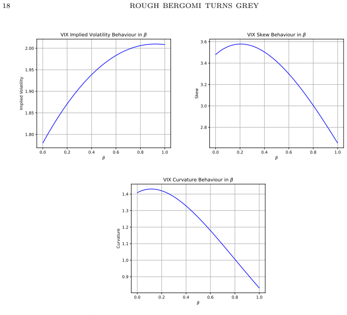
The central claim is that the system (2.9), with $dS_t/S_t = \sqrt{V_t}(\rho dB_t + \sqrt{1-\rho^2}dW_t)$ and $V_t = \xi_0(t)\,\mathcal{E}^{\lozenge}(\eta\sqrt{Y_\beta}B^H_t)$, where $B^H$ is a Riemann-Liouville fractional Brownian motion and $Y_\beta$ an independent M-Wright variable, preserves self-similarity and stationary increments while letting VIX marginals depart from log-normality. By Lemma 2.3 the grey noise admits the representation $B^{\beta,\alpha}_t \stackrel{d}{=} \sqrt{Y_\beta}B^{\alpha/2}_t$, so the model is exactly rough Bergomi with volatility of volatility randomised by $Y_\beta$. The paper proves the stock price is a true martingale for $\rho\le 0$, derives explicit VIX and VIX-futures expressions and bounds, computes the Malliavin derivatives that drive the asymptotics, and obtains small-time at-the-money limits for the VIX level, skew and curvature (Proposition 4.2) and for the SPX skew (Proposition 4.6). It then calibrates to market data and reports that the ATM VIX moments alone yield $\beta^*=1$, while a full-smile grid search gives $(H,\beta,\eta)=(0.015,0.11,2)$ for the VIX and $\eta=0.42$, $\rho=-1$ for the joint fit, which the authors describe as not particularly accurate, with the short-dated SPX skew the main miss.
Load-bearing premise
The load-bearing premise is that the small-time asymptotic formulas (Propositions 4.2 and 4.6, derived as $T\downarrow0$) are accurate enough at the one-month market maturity $T=0.094$ used in the calibration, since the paper provides no finite-maturity Monte Carlo validation of those formulas.
Editorial extensions
If this is right
- The VIX smile under gBergomi can slope upward, because VIX squared is no longer a near-log-normal conditional expectation and the M-Wright mixing injects skewness and excess kurtosis into VIX marginals.
- The small-time limits in Propositions 4.2 and 4.6 give a parameter recipe: VIX ATM level, skew and curvature fix $(H,\beta,\eta)$ through $J_1,J_2,J_3$, and the SPX ATM skew then fixes $\rho$, allowing calibration without Monte Carlo.
- Since the discounted stock price is a true martingale for $\rho\le 0$ and its running supremum has finite expectation, European option prices under (2.9) are arbitrage-free and numerically well behaved.
- The paper's own calibration shows two regimes: ATM VIX moments alone return $\beta^*=1$ (the log-normal case), while a full VIX-smile search gives a strongly non-Gaussian $\beta=0.11$; the joint SPX/VIX fit is not yet accurate, with the short-dated SPX skew the main miss.
- The VIX-futures upper and lower bounds in Proposition 2.10, together with the Markovian approximation in Appendix A, provide practical pricing shortcuts for longer maturities.
Reading between the lines
- Because $\beta$ and $\eta$ both scale the effective volatility of volatility, ATM level-skew-curvature data cannot separate them; a natural fix is to calibrate $\beta$ from the full VIX smile or from tail statistics such as those in Appendix B.
- The representation $B^{\beta,\alpha}_t=\sqrt{Y_\beta}B^{\alpha/2}_t$ suggests a latent-factor reading: $Y_\beta$ is a static volatility-of-volatility shock, so the model should be testable by comparing option-implied moments of VIX with the moment structure $\Gamma(1+\beta k/2)$ inherited from the M-Wright law.
- The short-maturity SSR limit $H+\tfrac32$ derived in Section 2.4 offers an out-of-sample check: if observed skew-stickiness at short maturities contradicts the calibrated $H$, the model cannot simultaneously match level and dynamics, pointing to the same tension seen in multifactor rough models.
Signed reviews
Editorial analysis
A structured set of objections, weighed in public.
Referee Report
Summary. The paper introduces the 'grey Bergomi' (gBergomi) model, in which the Gaussian driver of rough Bergomi is replaced by a generalized grey Brownian motion, adding a parameter β that makes the VIX marginals non-log-normal while retaining self-similarity and stationary increments. The authors derive the VIX representation, VIX futures bounds, Malliavin-derivative-based small-time asymptotics for both VIX and SPX implied volatilities, and numerical schemes based on truncated Cholesky and Markovian approximations. They then calibrate the model to SPX and VIX options data with maturity T=0.094 and claim that the model is a viable candidate for the joint SPX/VIX calibration problem. The mathematical framework and formulae are the main contribution; the empirical support for the headline claim is the weakest part of the manuscript.
Significance. If the model and its formulae are correct, this is a useful contribution to the rough-volatility literature: it provides a tractable non-log-normal generalization of rough Bergomi, with semi-closed VIX expressions, explicit VIX futures bounds, and Malliavin-based asymptotic smile formulas that reduce to known rough Bergomi results when β=1. The derivation of the VIX formula in Proposition 2.8 and the asymptotic formulas in Propositions 4.2 and 4.6 are consistent with the cited framework and appear algebraically sound. The calibration section, however, does not support the paper's central claim that gBergomi is a viable joint SPX/VIX calibration model: the unconstrained fit returns β*=1, the non-log-normal fit is obtained only after fixing parameters, and the SPX fit is acknowledged to be poor. The manuscript also contains the kernel of a finite-T validation problem, since small-time asymptotic limits are applied at a one-month maturity without checking their accuracy. These issues are fixable, but they currently prevent the empirical claim from being established.
major comments (4)
- [Section 5, Propositions 4.2 and 4.6] The calibration is built on T↓0 asymptotic limits applied to market options with maturity T=0.094, but the paper provides no finite-T Monte Carlo comparison, error bound, or convergence-rate estimate for these asymptotics. The reported optima (H*,β*,η*,ρ*)=(0.054,1,0.468,-1) and the later grid values (H,β,η,ρ)=(0.015,0.11,0.42,-1) are obtained entirely from these limits, so the empirical support for the joint-calibration claim depends on an unvalidated bridge between the asymptotics and the data. Remark 5.1 itself acknowledges that the low fitted η may be an artefact of not calibrating to one-day VIX options, which reinforces the need for a finite-T check.
- [Section 5 and Abstract] The abstract's claim that gBergomi 'breaks away from the log-Normal assumption' and is a viable joint SPX/VIX calibration model is not supported by the paper's own calibration results. The unconstrained optimization returns β*=1, which is exactly the log-normal rough Bergomi case, and the only non-log-normal calibration (β=0.11) is obtained by fixing η and grid-searching (H,β). After that procedure, Figure 8 shows a visibly poor SPX fit and the text states that the model 'does not achieve a particularly accurate fit, especially with respect to the short-dated skew'. The empirical evidence therefore does not establish the central claim; at most it shows that a generalized specification can produce a non-log-normal VIX smile when the parameters are constrained.
- [Remark 5.2] The paper acknowledges that β and η play similar roles and that one can fit the SPX smile with several (β,η) combinations if the VIX smile calibration is ignored. This implies that β is not identified from SPX options alone, which weakens the paper's claim that the non-log-normal feature is a genuine and separately estimable advantage of gBergomi. The manuscript should either provide an identification analysis, for example through the joint VIX and SPX fit, or explicitly limit the claim to the VIX marginals rather than to the joint calibration problem.
- [Section 4.2, proof of Proposition 4.6] The proof invokes 'reverse Fatou's lemma' to conclude that condition (iv), limsup_{T↓0} E[(sqrt(V_T/V_0)-1)^2]=0, follows from almost-sure continuity of V_t. Reverse Fatou requires a uniform integrability or domination argument, and none is supplied. Since condition (iv) is one of the hypotheses imported from [44, Proposition 5.1] that justify the SPX skew asymptotics used in the calibration, this is a load-bearing gap in the proof as written; please add the missing L^2 domination estimate or replace the argument with a direct bound.
minor comments (4)
- [Figure 2] Both panels of Figure 2 use the legend entry 'ggBergomi' where 'gBergomi' is intended; this typo appears twice.
- [Algorithm 3.1, step (iv)] The trapezoidal sum in step (iv) uses Q^2_{T,τ_j} but the grid {τ_j}_{j=0,...,N} is introduced only implicitly in step (i); the notation should be aligned so that the index range and the quadrature weights are unambiguous.
- [Section 2.2, around (2.9)] The correspondence between the generalized grey Brownian motion parameter α and the Hurst parameter H (α=2H) is stated only after the Riemann-Liouville replacement; stating it explicitly at the point of the replacement would improve readability.
- [Appendix B] The empirical normality tests are applied to VIX log-returns, while the model implication discussed in the introduction concerns the squared VIX being close to log-normal. The connection between these two objects should be stated explicitly so that the reader can see why the tests are evidence against the rBergomi VIX marginal assumption.
Circularity Check
No significant circularity: the gBergomi pricing and asymptotic results are derived from the model dynamics, and Section 5 is an honest calibration rather than a prediction forced by construction.
full rationale
The derivation chain is self-contained with respect to the model specification. System (2.9) defines the gBergomi variance as V_t = ξ0(t) E♦(η sqrt(Yβ) B^H_t); Proposition 2.8 derives the VIX squared as an integral of conditional expectations of this variance, Proposition 2.9 gives the forward variance, and Proposition 2.10 provides futures bounds. The small-time asymptotic results in Propositions 4.2 and 4.6 are not assumed: they are obtained by checking the general Malliavin-derivative assumptions from the published framework [44] and computing the gBergomi-specific quantities J1, J2, J3 and E[D_s V_u] from the model's Malliavin derivatives (4.1). The citation of [44] is load-bearing in the proof but is an independent general theorem whose assumptions here are verified in Lemmas 4.4 and 4.5, so it does not convert the argument into a self-citation loop. The calibration in Section 5 fits model-implied ATM level, skew, and curvature to market VIX data and then to SPX skew; Figures 7 and 8 display in-sample fits, and the paper explicitly reports the unconstrained optimum beta*=1 and the poor SPX fit. Weak empirical support for the joint-calibration claim, and the use of T down to 0 asymptotics at T=0.094 without finite-T validation, are correctness and robustness concerns, not circularity. No fitted quantity is relabelled as a prediction, and no result is equivalent to its inputs by construction.
Assumptions & free parameters
free parameters (5)
- H (Hurst exponent) =
0.054 (first calibration), 0.015 (VIX smile grid search)
- beta (grey parameter) =
1 (first calibration), 0.11 (grid search)
- eta (vol-of-vol) =
0.468 (first calibration), 2 (grid search), 0.4 to 0.42 (joint fit)
- rho (correlation) =
-1
- Arctan smoothing parameters (a,b,c,d) =
1.913, 0.746, -2.113, 0.761
assumptions (5)
- standard math Lemma 2.3: the generalised grey Brownian motion satisfies B^{beta,alpha}_t = sqrt(Y_beta) B^{alpha/2}_t with Y_beta an independent M-Wright random variable (Proposition 3 in [50]).
- domain assumption The variance process V is in the domain D of Malliavin calculus and satisfies the Lp bounds and continuity assumptions of [44, Proposition 1].
- standard math Clark-Ocone formula gives the martingale representation used for VIX and SPX futures in Section 4.
- domain assumption Risk-neutral valuation: VIX squared equals the conditional expectation of integrated variance over one month, and the discounted stock price is a true martingale for rho <= 0.
- domain assumption The Yahoo Finance market data from 26/10/2024 is representative, and the arctan interpolation preserves the true ATM level, skew and curvature.
Cite this review
Pith. "Pith review of Rough Bergomi turns grey." pith.science (2026). https://pith.science/paper/PAD42SYL
@misc{pith2026250508623,
  author       = {Pith},
  title        = {Pith review of: Rough Bergomi turns grey},
  year         = {2026},
  howpublished = {\url{https://pith.science/paper/PAD42SYL}},
  note         = {Machine review of arXiv:2505.08623}
}
read the original abstract
We propose a tractable extension of the rough Bergomi model, replacing the fractional Brownian motion with a generalised grey Brownian motion, which we show to be reminiscent of models with stochastic volatility of volatility. This extension breaks away from the log-Normal assumption of rough Bergomi, thereby making it a viable suggestion for the Equity Holy Grail -- the joint SPX/VIX options calibration. For this new (class of) model(s), we provide semi-closed and asymptotic formulae for SPX and VIX options and show numerically its potential advantages as well as calibration results.
Figures


Figures from the paper (8 more)



Reference graph
Works this paper leans on
-
[1]
E. Abi Jaber , The characteristic function of Gaussian stochastic volatility models: an analytic expression, Finance and Stochastics, 26 (2022), p. 733–769
work page 2022
-
[2]
State spaces of multifactor approximations of nonnegative Volterra processes
E. Abi Jaber, C. Bayer, and S. Breneis, State spaces of multifactor approximations of nonnegative Volterra processes, 2024. arXiv:2412.17526
work page Pith review arXiv 2024
-
[3]
E. Abi Jaber and O. El Euch, Multifactor approximation of rough volatility models, SIAM Journal on Financial Mathematics, 10 (2019), pp. 309–349
work page 2019
-
[4]
M. Abramowitz and I. Stegun , Handbook of Mathematical Functions, Dover, 1965
work page 1965
- [5]
-
[6]
E. Al`os and D. G. Lorite, Malliavin Calculus in Finance: Theory and Practice , CRC Press, 2021
work page 2021
-
[7]
F. J. Anscombe and W. J. Glynn , Distribution of the kurtosis statistic b2 for Normal samples , Biometrika, 70 (1983), p. 227
work page 1983
-
[8]
P. Bank, C. Bayer, P. K. Friz, and L. Pelizzari , Rough PDEs for local stochastic volatility models, Mathematical Finance, (2023)
work page 2023
Show all 56 references
-
[9]
O. E. Barndorff-Nielsen and A. E. Veraart, Stochastic volatility of volatility and variance risk premia, Journal of Financial Econometrics, 11 (2012), pp. 1–46. ROUGH BERGOMI TURNS GREY 23
2012
-
[10]
Bayer and S
C. Bayer and S. Breneis , Markovian approximations of stochastic Volterra equations with the fractional kernel, Quantitative Finance, 23 (2023), pp. 53–70
2023
-
[11]
Bayer, P
C. Bayer, P. Friz, and J. Gatheral , Pricing under rough volatility , Quantitative Finance, 16 (2015), pp. 887–904
2015
-
[12]
Bennedsen, A
M. Bennedsen, A. Lunde, and M. S. Pakkanen , Hybrid scheme for Brownian semistationary processes, Finance and Stochastics, 21 (2017), p. 931–965
2017
-
[13]
Bergomi, Smile dynamics II , Risk Magazine, October (2005)
L. Bergomi, Smile dynamics II , Risk Magazine, October (2005)
2005
-
[14]
Bergomi, Smile dynamics IV , Risk Magazine, (2009)
L. Bergomi, Smile dynamics IV , Risk Magazine, (2009)
2009
-
[15]
Bourgey, S
F. Bourgey, S. De Marco, and J. Delemotte, Smile dynamics and rough volatility, ssrn:4911186, (2024)
2024
-
[16]
Bourgey, S
F. Bourgey, S. D. Marco, and J. Delemotte , Yet another analysis of the SP500 at-the-money skew: crossover of different power-law behaviours , ssrn:4911186, (2024)
2024
-
[17]
Carmona, L
P. Carmona, L. Coutin, and G. Montseny, Approximation of some Gaussian processes, Statistical Inference for Stochastic Processes, 3 (2000), pp. 161–171
2000
-
[18]
Comte and E
F. Comte and E. Renault , Long memory continuous time models , Journal of Econometrics, 73 (1996), pp. 101–149
1996
-
[19]
J. L. da Silva and M. Erraoui , Singularity of generalized grey Brownian motions with different parameters, Stochastic Analysis and Applications, 36 (2018), pp. 726–732
2018
-
[20]
, Singularity of generalized grey Brownian motion and time-changed Brownian motion , AIP Conference Proceedings, 2286 (2020)
2020
-
[21]
D’Agostino and E
R. D’Agostino and E. S. Pearson , Tests for departure from Normality: empirical results for the distributions of b2 and √b1, Biometrika, 60 (1973), p. 613
1973
-
[22]
R. B. D’Agostino, An omnibus test of Normality for moderate and large size samples , Biometrika, 58 (1971), p. 341
1971
-
[23]
R. B. D’Agostino, A. Belanger, and R. B. D’Agostino Jr., A suggestion for using powerful and informative tests of Normality , The American Statistician, 44 (1990), p. 316
1990
-
[24]
Djehiche and M
B. Djehiche and M. Eddahbi , Hedging options in market models modulated by the fractional Brownian motion, Stochastic Analysis and Applications, 19 (2001), pp. 753–770
2001
-
[25]
El Euch and M
O. El Euch and M. Rosenbaum , Perfect hedging in rough Heston models , The Annals of Applied Probability, 28 (2018), pp. 3813–3856
2018
-
[26]
, The characteristic function of rough Heston models, Mathematical Finance, 29 (2019), pp. 3– 38
2019
-
[27]
Fenton, The sum of log-Normal probability distributions in scatter transmission systems , IEEE Transactions on Communications, 8 (1960), pp
L. Fenton, The sum of log-Normal probability distributions in scatter transmission systems , IEEE Transactions on Communications, 8 (1960), pp. 57–67
1960
-
[28]
H. Fink, C. Kl ¨uppelberg, and M. Z ¨ahle, Conditional distributions of processes related to frac- tional Brownian motion , Journal of Applied Probability, 50 (2013), pp. 166–183
2013
-
[29]
Fouque and Y
J.-P. Fouque and Y. F. Saporito , Heston stochastic vol-of-vol model for joint calibration of VIX and S&P 500 options , Quantitative Finance, 18 (2018), pp. 1003–1016
2018
-
[30]
Friz and J
P. Friz and J. Gatheral , Computing the SSR , Quantitative Finance, (2025), pp. 1–10
2025
-
[31]
Fukasawa, Asymptotic analysis for stochastic volatility: martingale expansion , Finance and Stochastics, 15 (2011), pp
M. Fukasawa, Asymptotic analysis for stochastic volatility: martingale expansion , Finance and Stochastics, 15 (2011), pp. 635–654
2011
-
[32]
Gassiat, On the martingale property in the rough Bergomi model , Electronic Communications in Probability, 24 (2019), pp
P. Gassiat, On the martingale property in the rough Bergomi model , Electronic Communications in Probability, 24 (2019), pp. 1–9
2019
-
[33]
Gatheral, T
J. Gatheral, T. Jaisson, and M. Rosenbaum, Volatility is rough, Quantitative Finance, 18 (2018), pp. 933–949
2018
-
[34]
Gatheral, P
J. Gatheral, P. Jusselin, and M. Rosenbaum , The quadratic rough Heston model and the joint S&P 500/VIX smile calibration problem , Risk.net, (2020)
2020
-
[35]
Gerhold, J
S. Gerhold, J. Pachschw ¨oll, and J. Ruf , On the integrability of the supremum of stochastic volatility models and other martingales , arXiv:2412.15746, (2024)
2024
-
[36]
Goutte, A
S. Goutte, A. Ismail, and H. Pham , Regime-switching stochastic volatility model: estimation and calibration to VIX options , Applied Mathematical Finance, 24 (2017), pp. 38–75
2017
-
[37]
Guyon and J
J. Guyon and J. Lekeufack, Volatility is (mostly) path-dependent, Quantitative Finance, 23 (2023), pp. 1221–1258
2023
-
[38]
Horvath, A
B. Horvath, A. Jacquier, and P. Tankov , Volatility options in rough volatility models , SIAM Journal on Financial Mathematics, 11 (2020), pp. 437–469. 24 ROUGH BERGOMI TURNS GREY
2020
-
[39]
Horvath, A
B. Horvath, A. Muguruza, and M. Tomas , Deep learning volatility , Quantitative Finance, 21 (2021), pp. 11–27
2021
-
[40]
Huang, C
D. Huang, C. Schlag, I. Shaliastovich, and J. Thimme , Volatility-of-volatility risk, Journal of Financial and Quantitative Analysis, 54 (2019), pp. 2423–2452
2019
-
[41]
H. E. Hurst , Long-term storage capacity of reservoirs , Transactions of the American Society of Civil Engineers, 116 (1951), pp. 770–799
1951
-
[42]
O. C. Ibe, Markov Processes for Stochastic Modeling, Second Edition , Academic Press, 2013
2013
-
[43]
Jacquier, C
A. Jacquier, C. Martini, and A. Muguruza , On VIX Futures in the rough Bergomi model , Quantitative Finance, 18 (2018), pp. 45–61
2018
-
[44]
Jacquier, A
A. Jacquier, A. Muguruza, and A. Pannier , Rough multifactor volatility for SPX and VIX options, Advances in Applied Probability, (2025), pp. 1–42
2025
-
[45]
J. Jia, Z. Wang, X. Huang, and Y. Wei , Some remarks on estimate of Mittag-Leffler function , Journal of Function Spaces, 2019 (2019), pp. 1–9
2019
-
[46]
A. N. Kolmogorov, Wienersche Spiralen und einige andere interessante Kurven im Hilbertschen Raum, Acad. Sci. URSS (NS), 26 (1940), pp. 115–118
1940
-
[47]
Lions and M
P.-L. Lions and M. Musiela , Correlations and bounds for stochastic volatility models , Annales de l’Institut Henri Poincar´ e C, Analyse non lin´ eaire, 24 (2007), pp. 1–16
2007
-
[48]
B. B. Mandelbrot and J. W. Van Ness , Fractional Brownian motions, fractional noises and applications, SIAM review, 10 (1968), pp. 422–437
1968
-
[49]
Mura and F
A. Mura and F. Mainardi , A class of self-similar stochastic processes with stationary increments to model anomalous diffusion in Physics , Integral Transforms and Special Functions, 20 (2009), pp. 185–198
2009
-
[50]
Mura and G
A. Mura and G. Pagnini , Characterizations and simulations of a class of stochastic processes to model anomalous diffusion , Journal of Physics A, 41 (2008), p. 41
2008
-
[51]
Nualart, The Malliavin Calculus and Related Topics , Springer-Verlag, 2006
D. Nualart, The Malliavin Calculus and Related Topics , Springer-Verlag, 2006
2006
-
[52]
Pipiras and M
V. Pipiras and M. S. Taqqu, Are classes of deterministic integrands for fractional Brownian motion on an interval complete? , Bernoulli, 7 (2001), p. 873
2001
-
[53]
L. C. G. Rogers , Arbitrage with fractional Brownian motion , Mathematical Finance, 7 (1997), pp. 95–105
1997
-
[54]
S. E. Rømer, Empirical analysis of rough and classical stochastic volatility models to the SPX and VIX markets, Quantitative Finance, 22 (2022), pp. 1805–1838
2022
-
[55]
Saichev and W
A. Saichev and W. Woyczynski, Models of anomalous diffusion: the subdiffusive case , Physica A, 349 (2005), pp. 375–420
2005
-
[56]
Q. Zhu, G. Loeper, W. Chen, and N. Langren ´e, Markovian approximation of the rough Bergomi model for Monte Carlo option pricing , Mathematics, 9 (2021), p. 528. Appendix A. Markovian Approximation of grey Bergomi Since the variance process in gBergomi is not Markovian, simula...
2021
Reviewed August 15, 2026 · model on record in the stance chip above.
Discussion (0). Continue with ORCID to comment.