Gaussian Process Differential Ensembles for Joint Inference on Curves, Derivatives, and Integrals
Pith reviewed 2026-06-26 07:40 UTC · model grok-4.3
The pith
Anchored Gaussian process differential ensembles embed a curve in a joint state with its derivatives and integrals, separating boundary uncertainty from the main covariance.
A machine-rendered reading of the paper's core claim, the machinery that carries it, and where it could break.
Core claim
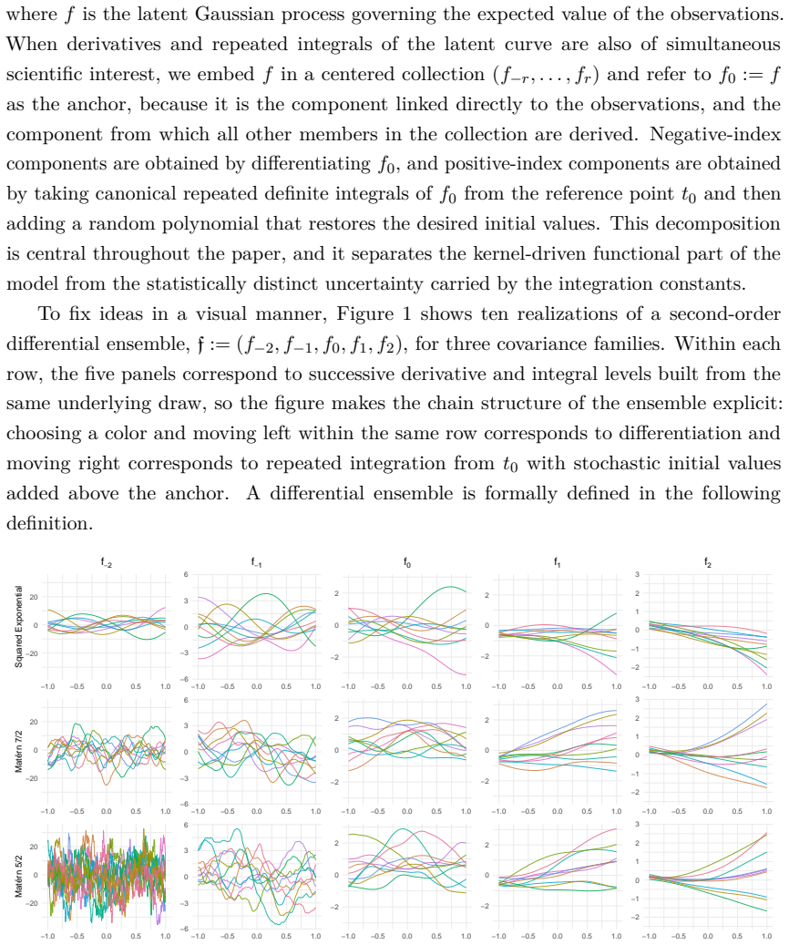
Anchored Gaussian process differential ensembles embed an anchor f0 in a joint Gaussian state together with its mean-square derivatives and repeated integrals; integral levels receive explicit Gaussian integration constants. The construction separates the anchor-induced covariance from the finite-dimensional boundary uncertainty and shows why observations of the anchor alone cannot identify the independent integration constants. For stationary one-dimensional kernels the ensemble is realized by a transformed Hilbert-space Gaussian-process approximation that applies the derivative and integral operators to Laplacian-Dirichlet basis functions while retaining the integration-constant covariance
What carries the argument
The anchored Gaussian process differential ensemble: a joint Gaussian state that augments an observed anchor function with its mean-square derivatives and repeated integrals, each integral level carrying an explicit Gaussian integration constant.
If this is right
- Joint posterior inference becomes available for any functional of the coupled state, such as turning-point locations or kinematic summaries.
- Derivative-aware calibration recovers derivative posteriors more accurately than anchor-only calibration while leaving anchor and integral summaries unchanged.
- Operator-level approximation bounds and conditional finite-grid posterior convergence hold for the Hilbert-space realization.
- Anchor-only data leave the integration constants unidentified, as shown by the explicit separation of covariance sources.
Where Pith is reading between the lines
- The same separation of boundary uncertainty could be tested in non-stationary or multi-dimensional kernels by replacing the Laplacian-Dirichlet basis with an appropriate eigenbasis.
- The explicit integration constants supply a natural route to uncertainty propagation when the model is embedded inside larger differential-equation or physics simulators.
- Because the construction is kernel-agnostic at the level of the joint state, it could be paired with any existing Gaussian-process approximation technique that admits derivative and integral operators.
Load-bearing premise
The joint ensemble can be computed exactly for stationary one-dimensional kernels by applying derivative and integral operators to a Laplacian-Dirichlet basis while preserving the integration-constant covariance.
What would settle it
A finite-grid simulation in which the marginal posterior variance of the integration constants changes when the anchor is observed alone, contrary to the claimed separation between anchor-induced covariance and finite-dimensional boundary uncertainty.
Figures
read the original abstract
Functional data are often modeled through one likelihood-linked curve, while the scientific target is a larger state containing rates, accumulated quantities, boundary values, or nonlinear functionals of several linked levels. These targets require more than smoothing the observed curve: derivative uncertainty, cross-level covariance, and integration constants must be handled jointly. We introduce anchored Gaussian process differential ensembles, embedding an anchor \(f_0\) in a joint Gaussian state with its mean-square derivatives and repeated integrals. Integral levels add explicit Gaussian integration constants. This separates the anchor-induced covariance from finite-dimensional boundary uncertainty and clarifies why anchor-only observations do not identify independent integration constants. For stationary one-dimensional kernels, we compute the ensemble with a transformed Hilbert space Gaussian process approximation that applies derivative and integral operators to Laplacian--Dirichlet basis functions while retaining the integration-constant covariance exactly. We establish operator-level approximation bounds and conditional finite-grid posterior convergence. We introduce TARTARE, a target-aware calibration procedure for finite-rank differential ensemble approximations, to address derivative under-resolution by anchor-calibrated bases. In second-order simulations, derivative-aware calibration improves derivative posterior recovery relative to anchor-only calibration while preserving anchor and integral summaries. A motorcycle crash analysis illustrates coherent posterior inference on a coupled kinematic state and short-horizon turning-point functionals.
Editorial analysis
A structured set of objections, weighed in public.
Referee Report
Summary. The paper introduces anchored Gaussian process differential ensembles that embed an observed anchor curve f0 into a joint Gaussian state with its mean-square derivatives and repeated integrals, adding explicit Gaussian integration constants at integral levels. This construction separates anchor-induced covariance from finite-dimensional boundary uncertainty. For stationary one-dimensional kernels the ensemble is realized via a transformed Hilbert-space GP approximation that applies derivative and integral operators to Laplacian-Dirichlet eigenfunctions while retaining the integration-constant covariance exactly; operator-level approximation bounds and conditional finite-grid posterior convergence are established. A target-aware calibration procedure (TARTARE) is proposed to mitigate derivative under-resolution, and the method is illustrated on second-order simulations and a motorcycle-crash kinematic analysis.
Significance. If the exact-retention property and the accompanying bounds hold, the framework supplies a coherent joint posterior for curves, derivatives, integrals and boundary constants that is directly useful in functional data settings where multiple linked quantities are scientifically relevant. Explicit credit is due for the operator-level bounds, the finite-grid convergence result, and the reproducible simulation design that isolates the effect of derivative-aware versus anchor-only calibration.
major comments (3)
- [§4.1] §4.1 (transformed Hilbert-space approximation): the assertion that the integration-constant covariance is retained exactly after applying the derivative/integral operators to the Laplacian-Dirichlet basis must be accompanied by an explicit transformation rule and a separate verification that the Dirichlet boundary conditions leave the constant term unaffected; the operator bounds stated in the text do not automatically guarantee this finite-dimensional exactness, which is load-bearing for the separation argument and for the subsequent TARTARE calibration.
- [§5.2] §5.2 (TARTARE calibration): the simulation results report improved derivative posterior recovery under derivative-aware bases, yet the quantitative effect on the joint integral summaries (mean and variance) is not tabulated; without these numbers it is impossible to confirm that the calibration preserves the very integral-level summaries the method is designed to deliver.
- [Theorem 3] Theorem 3 (finite-grid posterior convergence): the proof sketch relies on the exact retention property; if that property holds only approximately, the convergence statement requires an additional error term that propagates the deviation in the integration-constant block into the joint posterior.
minor comments (2)
- [§2] Notation for the integration constants (denoted C_k in the text) should be introduced once in §2 and used consistently thereafter; occasional reuse of the symbol for different levels creates ambiguity.
- [Figure 4] Figure 4 (motorcycle analysis) lacks axis labels on the turning-point functional panels; the reader cannot verify the scale of the reported credible intervals without them.
Simulated Author's Rebuttal
We thank the referee for the careful and constructive review. We respond point-by-point to the major comments below.
read point-by-point responses
-
Referee: [§4.1] §4.1 (transformed Hilbert-space approximation): the assertion that the integration-constant covariance is retained exactly after applying the derivative/integral operators to the Laplacian-Dirichlet basis must be accompanied by an explicit transformation rule and a separate verification that the Dirichlet boundary conditions leave the constant term unaffected; the operator bounds stated in the text do not automatically guarantee this finite-dimensional exactness, which is load-bearing for the separation argument and for the subsequent TARTARE calibration.
Authors: We agree that the exact-retention claim requires an explicit rule and independent verification. The revised manuscript will add a dedicated paragraph in §4.1 giving the transformation rule for the integration-constant block under the derivative and integral operators and a short proof that the Dirichlet conditions leave the constant mode unaffected, using the fact that the constant lies in the kernel of the Laplacian-Dirichlet operator and is orthogonal to the eigenfunctions. This verification will be separate from the operator-norm bounds. revision: yes
-
Referee: [§5.2] §5.2 (TARTARE calibration): the simulation results report improved derivative posterior recovery under derivative-aware bases, yet the quantitative effect on the joint integral summaries (mean and variance) is not tabulated; without these numbers it is impossible to confirm that the calibration preserves the very integral-level summaries the method is designed to deliver.
Authors: We accept the point. The revised §5.2 will include a supplementary table reporting the posterior mean and variance of the integral summaries (both first and second integrals) under anchor-only and derivative-aware calibration, confirming that the integral-level quantities remain essentially unchanged while derivative recovery improves. revision: yes
-
Referee: [Theorem 3] Theorem 3 (finite-grid posterior convergence): the proof sketch relies on the exact retention property; if that property holds only approximately, the convergence statement requires an additional error term that propagates the deviation in the integration-constant block into the joint posterior.
Authors: Theorem 3 is stated under the exact-retention property. Once the explicit verification requested in the §4.1 comment is supplied, the property will be established as exact and the existing proof sketch will suffice. If the added verification were to reveal a small deviation, we would insert the corresponding propagation error term into the convergence statement. revision: partial
Circularity Check
No circularity: method builds on established GP operator theory with independent approximation bounds and convergence claims.
full rationale
The abstract and description present a new anchored GP differential ensemble construction that applies derivative/integral operators to Laplacian-Dirichlet bases for stationary kernels, with explicit claims of proving operator-level bounds and finite-grid convergence. No self-citations, self-definitional loops, or fitted parameters renamed as predictions appear in the provided text. The integration-constant retention is asserted as a proved property rather than defined into existence. This matches the default expectation of a self-contained derivation without reduction to inputs by construction.
Axiom & Free-Parameter Ledger
axioms (1)
- domain assumption Stationary one-dimensional kernels admit a transformed Hilbert space approximation via Laplacian-Dirichlet basis functions that preserves integration-constant covariance exactly under derivative and integral operators.
Reference graph
Works this paper leans on
-
[1]
\'A lvarez, M. A., D. Luengo, and N. D. Lawrence (2013). Linear latent force models using Gaussian processes. IEEE Transactions on Pattern Analysis and Machine Intelligence\/ 35\/ (11), 2693--2705
2013
-
[2]
Cahill, N., A. C. Kemp, B. P. Horton, and A. C. Parnell (2015). Modeling sea-level change using errors-in-variables integrated gaussian processes. The Annals of Applied Statistics\/ 9\/ (2), 547--571
2015
-
[3]
Cramer, H. and M. Leadbetter (1967). Stationary and related stochastic processes-sample function properties and their applications
1967
-
[4]
de Souza, C. P. E. and N. E. Heckman (2014). Switching nonparametric regression models. Journal of Nonparametric Statistics\/ 26\/ (4), 617--637
2014
-
[5]
Graepel, T. (2003). Solving noisy linear operator equations by gaussian processes: Application to ordinary and partial differential equations. In Proceedings of the 20th International Conference on Machine Learning , pp.\ 234--241
2003
-
[6]
Gulian, M., A. L. Frankel, and L. P. Swiler (2022). Gaussian process regression constrained by boundary value problems. Computer Methods in Applied Mechanics and Engineering\/ 388 , 114117
2022
-
[7]
Durrande, and A
Hensman, J., N. Durrande, and A. Solin (2018). Variational Fourier features for Gaussian processes. Journal of Machine Learning Research\/ 18\/ (151), 1--52
2018
-
[8]
Sans \'o , H
Holsclaw, T., B. Sans \'o , H. K. Lee, K. Heitmann, S. Habib, D. Higdon, and U. Alam (2013). Gaussian process modeling of derivative curves. Technometrics\/ 55\/ (1), 57--67
2013
-
[9]
Kimeldorf, G. S. and G. Wahba (1970). A correspondence between Bayesian estimation on stochastic processes and smoothing by splines. The Annals of Mathematical Statistics\/ 41\/ (2), 495--502
1970
-
[10]
Lange-Hegermann, M. (2021). Linearly constrained Gaussian processes with boundary conditions. In Proceedings of the 24th International Conference on Artificial Intelligence and Statistics , Volume 130 of Proceedings of Machine Learning Research , pp.\ 1090--1098. PMLR
2021
-
[11]
L \'a zaro-Gredilla, M. and A. R. Figueiras-Vidal (2009). Inter-domain gaussian processes for sparse inference using inducing features. In Advances in Neural Information Processing Systems 22 , pp.\ 1087--1095
2009
-
[12]
Liu, C.-H
Li, M., Z. Liu, C.-H. Yu, and M. Vannucci (2024). Semiparametric Bayesian inference for local extrema of functions in the presence of noise. Journal of the American Statistical Association\/ 119\/ (548), 3127--3140
2024
-
[13]
Liu, Z. and M. Li (2026). Optimal plug-in Gaussian processes for modeling derivatives. Journal of the American Statistical Association\/ . Advance online publication
2026
-
[14]
Matheron, G. (1973). The intrinsic random functions and their applications. Advances in Applied Probability\/ 5\/ (3), 439--468
1973
-
[15]
Murray-Smith, R. and B. A. Pearlmutter (2005). Transformations of gaussian process priors. In J. Winkler, M. Niranjan, and N. Lawrence (Eds.), Deterministic and Statistical Methods in Machine Learning , Volume 3635 of Lecture Notes in Computer Science , pp.\ 110--123. Berlin, Heidelberg: Springer
2005
-
[16]
Ramsay, J. O., G. Hooker, D. Campbell, and J. Cao (2007). Parameter estimation for differential equations: A generalized smoothing approach. Journal of the Royal Statistical Society: Series B (Statistical Methodology)\/ 69\/ (5), 741--796
2007
-
[17]
Ramsay, J. O. and B. W. Silverman (2005). Functional Data Analysis\/ (2 ed.). New York: Springer
2005
-
[18]
B \"u rkner, M
Riutort-Mayol, G., P.-C. B \"u rkner, M. R. Andersen, A. Solin, and A. Vehtari (2023). Practical hilbert space approximate bayesian gaussian processes for probabilistic programming. Statistics and Computing\/ 33\/ (1), 17
2023
-
[19]
S \"a rkk \"a , S. (2011). Linear operators and stochastic partial differential equations in Gaussian process regression. In Artificial Neural Networks and Machine Learning -- ICANN 2011 , Volume 6792 of Lecture Notes in Computer Science , pp.\ 151--158. Springer
2011
-
[20]
Silverman, B. W. (1985). Some aspects of the spline smoothing approach to non-parametric regression curve fitting. Journal of the Royal Statistical Society: Series B (Methodological)\/ 47\/ (1), 1--52
1985
-
[21]
Murray-Smith, W
Solak, E., R. Murray-Smith, W. Leithead, D. Leith, and C. Rasmussen (2002). Derivative observations in gaussian process models of dynamic systems. Advances in neural information processing systems\/ 15
2002
-
[22]
Solin, A. and S. S \"a rkk \"a (2020). Hilbert space methods for reduced-rank gaussian process regression. Statistics and Computing\/ 30\/ (2), 419--446
2020
-
[23]
Stan Modeling Language Users Guide and Reference Manual, Version 2.30
Stan Development Team (2026). Stan Modeling Language Users Guide and Reference Manual, Version 2.30
2026
-
[24]
Swain, P. S., K. Stevenson, A. Leary, L. F. Montano-Gutierrez, I. B. Clark, J. Vogel, and T. Pilizota (2016). Inferring time derivatives including cell growth rates using gaussian processes. Nature communications\/ 7\/ (1), 13766
2016
-
[25]
Wahba, G. (1978). Improper priors, spline smoothing and the problem of guarding against model errors in regression. Journal of the Royal Statistical Society: Series B (Methodological)\/ 40\/ (3), 364--372
1978
-
[26]
Williams, C. K. and C. E. Rasmussen (2006). Gaussian processes for machine learning . MIT press Cambridge, MA
2006
-
[27]
Yu, C.-H., M. Li, C. Noe, S. Fischer-Baum, and M. Vannucci (2023). Bayesian inference for stationary points in Gaussian process regression models for event-related potentials analysis. Biometrics\/ 79\/ (2), 629--641
2023
-
[28]
Yue, Y. R., D. Simpson, F. Lindgren, and H. Rue (2014). Bayesian adaptive smoothing splines using stochastic differential equations. Bayesian Analysis\/ 9\/ (2), 397--424
2014
-
[29]
Stringer, P
Zhang, Z., A. Stringer, P. Brown, and J. Stafford (2024). Model-based smoothing with integrated Wiener processes and overlapping splines. Journal of Computational and Graphical Statistics\/ 33\/ (3), 883--895
2024
discussion (0)
Sign in with ORCID, Apple, or X to comment. Anyone can read and Pith papers without signing in.