REVIEW 3 major objections 3 minor 13 references
An atlas of coronal electron density at 5Rs II: A spherical harmonic method for density reconstruction
T0 review · 3 major / 3 minor · reviewed 2026-08-14 · deepseek-v4-flash
Pith's one-line read This paper claims that coronal electron density can be reconstructed from coronagraph images by expanding the density in spherical harmonics on a shell at about 5 solar radii, assuming a radial corona above that height, and solving a…
desk verdict A genuinely new and efficient spherical-harmonic inversion trick for coronal tomography, with a heuristic regularization and an unresolved radial-falloff assumption that the real-data cross-spacecraft discrepancy (38%) keeps alive; worth a serious referee. read the letter →
The pith
A machine-rendered reading of the paper's core claim, the machinery that carries it, and where it could break.
The reading
What carries the argument
The central object is the precomputed line-of-sight integral of each spherical harmonic, $A_i = \sum_j g_j f(r_j) S_{ij}$, evaluated once for a fixed radial falloff $f(r) = (r_0/r)^\alpha$ with $\alpha = 2.2$. Because the corona is assumed radial above the height of interest, $A_i$ does not depend on the unknown density, so the brightness becomes a linear system $b = A c$. The coefficients $c$ are then found by noise-weighted regularized least squares, with a diagonal penalty $w_i = (l_i + |m_i|)/\sum_i(l_i + |m_i|)$ that increasingly damps high-order harmonics, and a two-parameter scan over the smoothing factor $\lambda$ and a minimum density threshold $\rho'$ sets the final smoothness and non-negativity.
What would settle it
Generate synthetic observations from a model in which the radial falloff differs between streamers and coronal holes, then reconstruct using the paper's fixed profile with $\alpha = 2.2$; if the streamer-belt density error exceeds the roughly 12% seen in the paper's own synthetic tests, the uniform-profile assumption fails. An independent check is to compare the reconstructed density at 5 solar radii with in situ density measurements from a spacecraft crossing that height.
Extended reading notes
Core claim
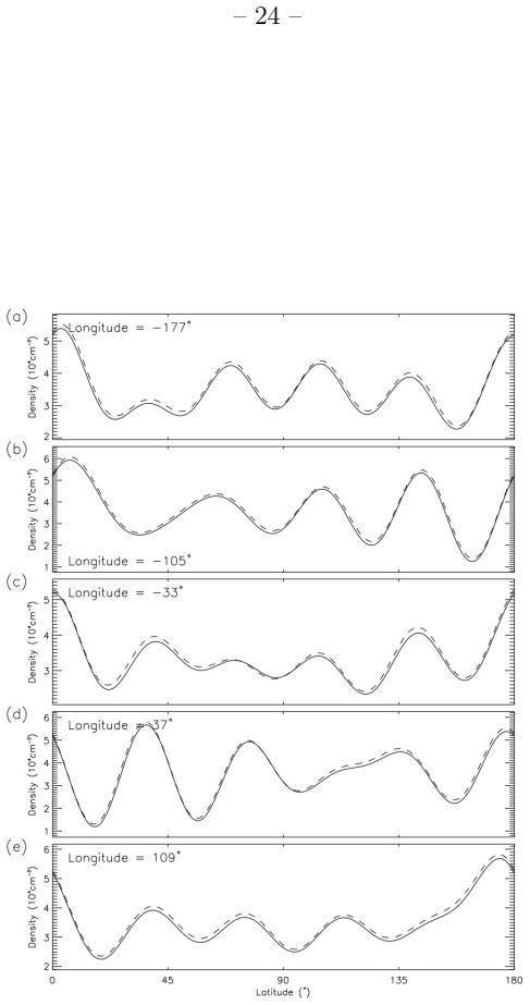
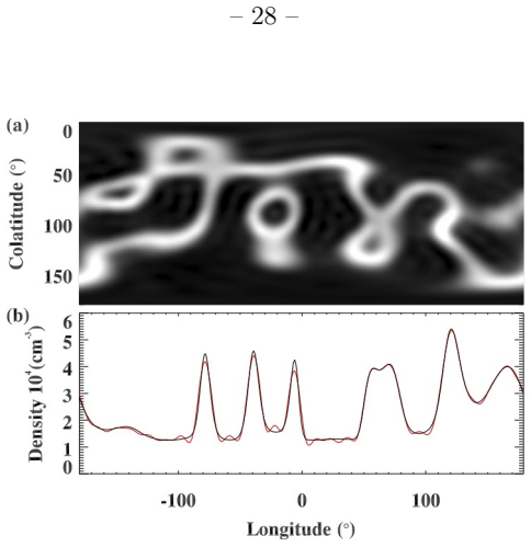
The central claim is that the assumption of a radially structured corona above the height of interest decouples the tomography problem: the line-of-sight summation for each spherical harmonic basis function, $A_i = \sum_j g_j f(r_j) S_{ij}$, depends only on geometry and the fixed radial profile $f(r) = (r_0/r)^\alpha$ with $\alpha = 2.2$, not on the unknown density. Once these $A_i$ are precomputed, the observed brightness is a linear combination $b = A c$, and the density is recovered by solving a noise-weighted, regularized least-squares problem whose diagonal penalty damps high-order harmonics and whose minimum-density threshold is selected by a two-parameter goodness-of-fit scan. In synthetic tests the reconstruction reaches 3.8% mean absolute fractional deviation for a harmonic-generated target and 12.3% for a narrowly ridged target after regularization, with no negative densities; with added noise and multi-day gaps the deviation stays near 14%. On real data from 2009/03/20 the method yields a streamer belt at 5.5 solar radii that is narrower and about half as dense as a previous reconstruction, with a 38% mean absolute fractional difference between the LASCO C2 and STEREO COR2 results.
Load-bearing premise
The load-bearing premise is that above the height of interest the corona is radially structured everywhere and that a single, uniform radial density falloff $f(r) = (r_0/r)^\alpha$ with $\alpha = 2.2$ describes the decrease at every longitude and latitude; if the true falloff varies in space, the separation of harmonics in the precomputed integrals is only approximate and the recovered coefficients are biased.
Editorial extensions
If this is right
- Routine long-term mapping becomes feasible: with integrations done once, a two-week reconstruction completes in minutes, enabling multi-year atlases of coronal density.
- The method's tolerance of several-day data gaps and 5% noise means degraded images can be discarded without destroying the reconstruction, simplifying processing pipelines.
- Regularization eliminates negative densities, a known problem in coronal tomography, at the cost of smoothness near the equator where gradients are sharpest.
- A time-dependent extension with harmonic coefficients varying in time is identified as the next step, but is found challenging, especially for step changes associated with coronal mass ejections.
Reading between the lines
- If the uniform radial falloff is genuinely wrong in a spatially varying way, the 38% difference between the two spacecraft may partly reflect that assumption rather than instrument calibration; an iterative scheme that updates $f(r)$ per region or per harmonic order would be a direct test.
- The same precomputation trick transfers to any basis that factorizes the line-of-sight integral, such as wavelet bases on the sphere, which the paper already suggests for the non-radial low corona.
- In situ density measurements from a spacecraft crossing the 5-solar-radii shell would give an independent, quantitative check of the radial-profile assumption and the reconstructed values.
- The reported downward revision of streamer density by roughly a factor of two relative to earlier work is an empirical claim that could be checked against simultaneous white-light eclipse measurements at the same height.
Signed reviews
Editorial analysis
A structured set of objections, weighed in public.
Referee Report
Summary. The manuscript presents a tomographic inversion method for white-light coronal observations at heights around 5 Rsun. The key idea is to represent the density on a spherical shell by spherical harmonics and, under the assumption of a radially structured corona with a uniform height profile f(r) = (r0/r)^alpha, to precompute line-of-sight integrations once per harmonic basis. The density reconstruction then reduces to a regularized linear least-squares fit, claimed to be very efficient. The method is tested on synthetic data from a simple spherical-harmonic density and from a more intricate, narrowly peaked distribution, with added noise and data gaps, and is applied to LASCO C2 and STEREO COR2 observations for March 2009. The paper concludes that the method is efficient, stable, and suitable for routine long-term coronal mapping.
Significance. If the efficiency and stability claims hold, the method could enable routine tomographic maps of the extended corona over long periods, which is valuable for solar-wind studies, space-weather applications, and linking coronal structure to in situ measurements. The manuscript has clear strengths: the linear algebra is transparent, the synthetic tests include a non-trivial target and explicitly test robustness to noise and large data gaps, and the real-data comparison is honest about the LASCO/COR2 discrepancy. However, the central assumption of a single, angle-independent radial falloff is only weakly validated, and the regularization parameter selection is heuristic. These issues do not invalidate the basic approach, but they need to be addressed before the long-term mapping claim is fully supported.
major comments (3)
- [Section 2.1, Eqs. (4)-(6)] The factorization that permits line-of-sight sums to be computed once per harmonic is exact only when f(r) in Eq. (3) is independent of longitude and latitude. If the radial falloff varies with structure, for example in streamers versus coronal holes, Eq. (4) contains cross terms and Eq. (6) with precomputed A_i is only approximate; the reconstructed coefficients then absorb the mismatch. The paper acknowledges this simplification, but the validation is not isolating. In Section 3, the synthetic data are generated with the non-uniform Doyle and Gibson radial profiles while the reconstruction assumes Eq. (2), yet the target is a smooth L=11 spherical harmonic with known order, so a slowly varying radial-profile error can be absorbed by the surface-density coefficients and long line-of-sight averages. I request a quantitative test that specifically varies the radial falloff with angular position, e.g., a streamer-like slower falloff and a coronal-hole-like faster falloff, and reconstructs with the uniform Eq. (2), reporting the resulting bias in density and in the coefficient estimates.
- [Section 7, Figs. 12-13] The real-data comparison reports a 38% mean absolute difference between the LASCO C2 and COR2 A reconstructions with an 81% correlation. This is a large discrepancy, and the manuscript does not quantify how much of it is caused by the assumed uniform f(r), by regularization choices, by calibration differences between instruments, or by temporal changes over the two-week interval. Since the stated goal is reliable maps over long time periods, this decomposition is important. A concrete improvement would be to apply the same reconstruction pipeline to synthetic data viewed from two different spacecraft with known instrumental offsets, or to cross-calibrate the two reconstructions against a common standard and state the residual attributable to the radial-profile assumption.
- [Section 5, Eq. (14) and Fig. 8] The selection of the regularization parameter lambda and the minimum density threshold rho' is defined by a heuristic: the 'optimal point' is halfway between the centroid of the low-chi region and the farthest boundary point, with the region itself set by the 15% percentile of chi. This is said to be based on 'tests using several different density distributions,' but no sensitivity analysis is shown. Because the final density maps depend on these two parameters, the manuscript should either justify the heuristic with a reproducible criterion (for example, an L-curve or generalized cross-validation) or demonstrate that reconstructions are insensitive to the exact choice within the flat region of Fig. 8. Without this, the regularization step is not fully specified.
minor comments (3)
- [Appendix, equations] The appendix restarts equation numbering at (1), which creates ambiguity when the text refers to 'equation 5 of section 2.1' (main-text Eq. 5) while the appendix also has its own Eq. (5). Renumbering the appendix as (A1), (A2), etc. would remove this confusion.
- [Section 5, Fig. 8 caption and text] The description of the white contour as 'the 15% percentile minimum value of chi' is ambiguous: it is not clear whether the shaded region contains values below the 15th percentile of chi or above it. Please clarify the definition in the text or caption.
- [Section 7, line after Eq. (12)] The phrase 'the A^T A covariance matrix is pre-computed' refers to the regularized normal equations; the word 'covariance' is nonstandard here and could be replaced by 'normal-equations matrix' for clarity.
Circularity Check
No significant circularity: the spherical-harmonic inversion is a genuine separation-of-variables derivation, and the synthetic tests use independently constructed target densities.
full rationale
The paper's central claim is that under the explicit assumption of a radial corona with a height-only falloff f(r), the line-of-sight brightness integral separates over spherical-harmonic basis functions (Eqs. 1-6). This is a mathematical identity, not an input dressed as a prediction: Eq. (6) follows from Eq. (5) by linearity of integration, and f(r) is an assumed profile (Eq. 2) rather than a parameter fitted to the brightness that is later 'predicted'. The synthetic tests use target densities constructed independently: the simple SH-based target is admitted to be a weak test, and the more intricate target (Eq. 10) is not SH-limited and is reconstructed with L=25 without knowing the input order. The reconstructed brightness matching observed brightness is a least-squares goodness-of-fit, not an independent prediction. The regularization parameters lambda and rho prime are tuned to the data but are nuisance parameters; the paper does not present them as derived physical predictions. The self-citations (Paper I for calibration/processing, and Morgan & Habbal 2010 for streamer morphology) are not used to justify the core inversion identity, so no circularity score is warranted.
Assumptions & free parameters
free parameters (3)
- Regularization parameter λ =
1.74e3 (synthetic test), 6.2e4 (LASCO C2), 5.1e4 (COR2 A)
- Minimum density threshold ρ' =
10.4e3 cm^-3 (synthetic), 1.4e3 cm^-3 (LASCO C2), 6.5e3 cm^-3 (COR2 A)
- Spherical harmonic order L =
L=11 (simple test), L=25 (complex test), not specified for real data
assumptions (5)
- domain assumption The corona is radial above the height of interest r0.
- domain assumption A single uniform radial density profile f(r)=(r0/r)^α with α=2.2 applies everywhere above r0.
- domain assumption Line-of-sight integrations can be truncated at ±10 R⊙ with negligible error.
- standard math Spherical harmonics form a complete basis for density on a sphere.
- domain assumption Observed K-coronal brightness is a linear integral of electron density times known Thomson scattering factors.
Cite this review
Pith. "Pith review of An atlas of coronal electron density at 5Rs II: A spherical harmonic method for density reconstruction." pith.science (2026). https://pith.science/paper/PNQKZIJN
@misc{pith2026190807866,
  author       = {Pith},
  title        = {Pith review of: An atlas of coronal electron density at 5Rs II: A spherical harmonic method for density reconstruction},
  year         = {2026},
  howpublished = {\url{https://pith.science/paper/PNQKZIJN}},
  note         = {Machine review of arXiv:1908.07866}
}
read the original abstract
This is the second of a series of three papers that present a methodology with the aim of creating a set of maps of the coronal density over a period of many years. This paper describes a method for reconstructing the coronal electron density based on spherical harmonics. By assuming a radial structure to the corona at the height of interest, line-of-sight integrations can be made individually on each harmonic basis prior to determining coefficients, i.e. the computationally-expensive integrations are calculated only once during initialization. This approach reduces the problem to finding the set of coefficients which best match the observed brightness using a regularized least-squares approach, and is very efficient. The method is demonstrated on synthetic data created from both a simple and an intricate coronal density model. The quality of reconstruction is found to be reasonable in the presence of noise and large gaps in the data. The method is applied to both LASCO C2 and STEREO COR2 coronagraph observations from 2009/03/20, and the results from both spacecraft compared. Future work will apply the method to large datasets.
Figures


Figures from the paper (10 more)




Reference graph
Works this paper leans on
-
[1]
1999, LAPACK Users’ Guide (SIAM)
Anderson, E., et al. 1999, LAPACK Users’ Guide (SIAM)
work page 1999
-
[2]
Arridge, S. R., & Schotland, J. C. 2009, Inverse Problems, 25, 123010
work page 2009
-
[3]
Aschwanden, M. J. 2011, Living Reviews in Solar Physics, 8, 5
work page 2011
-
[4]
2005, Geophysical Journal International, 163, 875
Chambodut, A., Panet, I., Mandea, M., Diament, M., Holschneider, M., & Jamet, O. 2005, Geophysical Journal International, 163, 875
work page 2005
-
[5]
G., Teriaca, L., & Banerjee, D
Doyle, J. G., Teriaca, L., & Banerjee, D. 1999, A&A, 349, 956
work page 1999
-
[6]
Frazin, R. A. 2000, ApJ, 530, 1026
work page 2000
-
[7]
A., Lamy, P., Llebaria, A., & V´ asquez, A
Frazin, R. A., Lamy, P., Llebaria, A., & V´ asquez, A. M. 2010, Sol. Phys., 265, 19
work page 2010
-
[8]
Gibson, S. E., Foster, D. J., Guhathakurta, M., Holzer, T., & St. Cyr, O. C. 2003, Journal of Geophysical Research (Space Physics), 108, 7
work page 2003
Show all 13 references
-
[9]
Y., Aides, A., & Davis, A
Levis, A., Schechner, Y. Y., Aides, A., & Davis, A. B. 2015, in 2015 IEEE International Conference on Computer Vision (ICCV), 3379–3387
2015
-
[10]
T., McElhinny, M
Merrill, R. T., McElhinny, M. W., & McFadden, P. L. 1996, MAGNETIC FIELD OF THE
1996
-
[11]
2015, ApJS, 219, 23
Morgan, H. 2015, ApJS, 219, 23
2015
-
[12]
Morgan, H., & Habbal, S. R. 2010, ApJ, 710, 1 Qu´ emerais, E., & Lamy, P. 2002, A&A, 393, 295
2010
-
[13]
A., & Wojak, J
Vibert, D., Peillon, C., Lamy, P., Frazin, R. A., & Wojak, J. 2016, Astronomy and Computing, 17, 144 – 35 – This manuscript was prepared with the AAS LATEX macros v5.2
2016
Reviewed August 14, 2026 · model on record in the stance chip above.
Discussion (0). Continue with ORCID to comment.