REVIEW 4 major objections 5 minor 1 cited by
ML-Driven Strong Lens Discoveries: Down to $\theta_E \sim 0.03''$ and $M_\mathrm{halo}< 10^{11} M_\odot$
T0 review · 4 major / 5 minor · reviewed 2026-08-06 · deepseek-v4-flash
Pith's one-line read The paper claims that machine-learned classifiers trained on realistic simulations can find gravitational lenses with Einstein radii down to about 0.03 arcseconds and halo masses below 10^11 solar masses, a regime that is effectively…
desk verdict A careful simulation-driven forecast of low-mass strong lenses with JWST, but the headline 100% purity is not demonstrated and one table contradicts another. read the letter →
The pith
A machine-rendered reading of the paper's core claim, the machinery that carries it, and where it could break.
The reading
What carries the argument
The machinery is a two-stage pipeline. First, a 'shielded' ResNet classifier scans image cutouts and assigns each a lens probability; it was trained on thousands of simulated images built from CosmoDC2 lens halos, VELA hydrodynamic source galaxies, and Sersic/environmental galaxies, with HST or JWST noise added during training. Second, a U-Net segmentation model takes ResNet-positive cutouts and predicts a per-pixel lens-location probability, so the lens position can be pinpointed. The forecasts that set the discovery rates use the CosmoDC2 halo catalog plus the Zahid et al. (2018) halo-mass-to-velocity-dispersion relation to convert halo masses into Einstein radii, and count lens-source overlap with three geometric methods: source in lens area, lens in source area, or either.
What would settle it
Run the trained RUN pipeline on a few square degrees of deep JWST imaging; if the yield of localized lenses with halo mass below $10^{11}M_\odot$ and Einstein radii between $0.02''$ and $0.05''$ is far below 1.1 per square degree at the claimed precision threshold, the forecast and transferability assumption fail.
Extended reading notes
Core claim
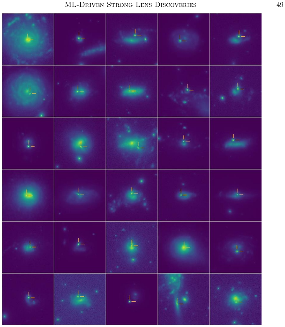
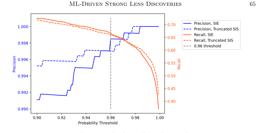
The central claim is that strong lens detection is no longer limited by human visual inspection or by Einstein radii large enough to show visible arcs: a shielded ResNet classifier trained on simulations with realistic hydrodynamic sources can identify lenses down to JWST's diffraction limit, and a U-Net can pinpoint their locations. On simulated JWST data with 10,000-second exposures, the ResNet achieves high classification accuracy for lenses with $0.02''<\theta_E<0.15''$, and the combined RUN pipeline reaches 100 percent pixel-level precision at a 0.96 ResNet threshold and a 0.72 U-Net threshold. Applied to real HST data, the conventional-lens model classified every test lens as a lens with high probability and identified two candidates missed by a crowdsourced citizen-science search. The authors conclude that the bottleneck is no longer finding candidate lenses but confirming them spectroscopically.
Load-bearing premise
The forecast numbers rest on the assumption that the simulated images, built from VELA sources, CosmoDC2 lenses, SIE mass profiles, and the JWST noise model, capture the appearance of real small-Einstein-radius lenses, and that the unmeasured halo-mass-to-velocity-dispersion relation below about 100 km/s used to convert halo mass into Einstein radius is roughly right.
Editorial extensions
If this is right
- Near-100 percent completeness and purity for conventional lenses means space-based surveys with HST, JWST, Roman, and Euclid can automate lens discovery instead of relying on human scanning.
- JWST should reveal about 17 lenses per square degree with halo mass below $10^{11}M_\odot$ and Einstein radii $0.02''$ to $0.05''$, with about 1.1 per square degree localized by the RUN pipeline at zero false positives.
- The two HST candidates show that even comprehensive crowdsourced searches miss discoverable lenses; machine learning can recover such systems.
- The low-mass lens population provides a new observational handle on CDM predictions for halo abundance below about $10^{11}M_\odot$.
Reading between the lines
- If real JWST images match the simulation inputs, then existing deep JWST surveys already contain these small lenses, and rerunning the trained pipeline on archival data is a direct test of the forecast.
- Because the halo-mass-to-velocity-dispersion relation is unconstrained below about 100 km/s, the forecast rates could shift by an order of magnitude; measuring that relation from dwarf-galaxy kinematics would firm up or revise the numbers.
- The same approach may extend to even smaller, effectively dark halos below $10^{10}M_\odot$ with higher-resolution instruments, since the lensing signal is not obscured by lens light.
- Multi-band imaging, by separating lens and source light, could help confirm small-Einstein-radius candidates and improve precision beyond single-band detection.
Editorial analysis
A structured set of objections, weighed in public.
Referee Report
Summary. The paper forecasts the number of strong gravitational lenses detectable with JWST, simulates lensed and unlensed images using CosmoDC2, JAGUAR/W18, and VELA sources, trains a shielded ResNet for three Einstein-radius ranges, and trains a U-Net to localize small-Einstein-radius lenses. The central new claims are that JWST can find ~17 deg^-2 lenses with 0.02''<θ_E<0.05'' and M_halo<10^11 M_sun using a ResNet, and that the combined ResNet+U-Net pipeline can localize ~1.1 deg^-2 of them at ~100% pixel-level precision (or ~7.0 deg^-2 at 99% precision). The paper also reports two new HST lens candidates missed by the Garvin et al. (2022) crowdsourcing search.
Significance. If the small-lens forecasts hold, this work opens a genuinely new observational regime: galaxy-scale strong lensing below θ_E≈0.03'' and M_halo≈10^11 M_sun would provide a new probe of low-mass dark matter halos. The simulation effort is unusually thorough for this type of forecast, and the k-fold VELA split, truncated-SIS test, environmental-galaxy variation, and real-HST validation for conventional lenses are genuine strengths. The two new HST candidates and the demonstration that Model 1a separates real lenses from non-lenses are concrete, falsifiable results that support the conventional-lens part of the paper. The small-lens part is scientifically important but currently rests on in-sample validation and unpropagated systematics.
major comments (4)
- [§3.3.3, Table 9 vs. Table 8] The forecast base for the headline bin is internally inconsistent. Table 8 states that the 0.02''<θ_E<0.05'' bin contains 240 lenses/deg^2 with M_halo<10^11 M_sun (the difference of the first two rows of Table 2), while Table 9 lists 490 lenses/deg^2 for the same bin and the same mass cut. Because the 17 and 1.1 deg^-2 numbers are derived from this bin, the authors must determine which base is correct, correct the affected tables/figures, and recompute the predicted yields.
- [§3.2.2.4, §4.2.2, Table 9, Abstract] The claim of ~100% precision for the 1.1/deg^2 (and 7.0/deg^2 at 99%) forecast is a validation-set zero-count statement, not a statistically supported field-deployment bound. With ~2000 Type-2 non-lenses, zero false positives gives a 95% upper limit of order 3.7 false positives (FPR≈0.0019); combined with the paper's own 1/3800 lens prior and a recall of ~0.67, the expected precision at the chosen ResNet threshold is not 100%. The paper itself computes a 5.56:1 FP:TP ratio at threshold 0.95 in §3.2.2.4, and the 0.96 and 0.72 thresholds were selected after inspecting the same validation set. The abstract and Table 9 should report a confidence interval for precision or an expected field precision under the stated prior, not a point value of 100% from zero counts.
- [§2.1.3, §2.3, §3.3.3] The headline yields (17, 7.0, and 1.1 deg^-2) are point estimates with no propagated uncertainty. The M_halo–σ relation of Zahid et al. (2018) is unconstrained below σ≈100 km/s, as the paper acknowledges in §2.3, and θ_E scales as σ^2; plausible changes in the normalization, slope, scatter, or low-σ behavior can shift the small-θ_E counts by an order of magnitude. The authors should provide credible intervals by varying the Z18 relation parameters, its scatter, and the VDF assumptions, and propagate these through Figure 21 and the U-Net recall factors.
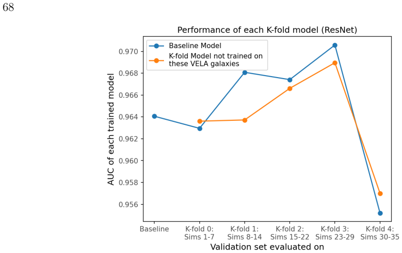
- [§3.1, §3.2.2, §4.2, §3.3.3] The small-lens completeness and purity used in the forecast are measured on simulations generated with the same source catalog (VELA), lens profile (SIE), PSF model, and noise model used to construct the forecast, and no real JWST small-θ_E validation exists. The k-fold VELA split and truncated-SIS tests are useful robustness checks, but they do not constrain performance on real JWST images with realistic PSF structure, blending, and source morphologies at θ_E≈0.03''. The deployment rates should be explicitly framed as simulation-based predictions, and a concrete validation path—such as a blinded injection test on real JWST imaging or a pilot search with spectroscopic follow-up—should be identified.
minor comments (5)
- [§3.1.5] The exposure times for Model 2a and Model 2b appear swapped in the text: Table 3 assigns 10,000 s to Model 2a (JWST-long) and 1,000 s to Model 2b (JWST-short), but §3.1.5 states texp=1000 s for Model 2a and texp=10,000 s for Model 2b.
- [§3.2.1.1, Table 6] Table 6 lists the recall at probability threshold 0.5 as 0.9034, which is an outlier relative to the neighboring thresholds (0.9824 and 0.9794) and inconsistent with the text's statement of 0.980 recall at a 0.5 threshold; this is likely a typographical error and should be corrected.
- [§3.2.2.4] The deployment calculation contains a wording error: after estimating 1.8 true positives and 10 false positives, the text says '1.8 are false positives,' but the context indicates it should read '1.8 are true positives.'
- [§4.2.2 and §4.3] The text claims zero false positives for the U-Net above threshold 0.72 in one place, while §4.2.2 reports one false positive at that threshold and Figure 25 shows a red point above the 0.72 line; the 'zero' claim should be restricted to the ResNet-filtered subset used for the final pipeline, or the count should be stated consistently.
- [Abstract and §3.2.2.2] The abstract describes going down to θ_E≲0.03'', but Figure 14 shows that recall degrades sharply toward θ_E=0.02'' (roughly 40% at threshold 0.5); the completeness caveat at the lowest Einstein radii should appear near the headline claim.
Circularity Check
No significant circularity: the lens forecasts are a forward model and the ML performance numbers are measured, not fitted parameters renamed as predictions.
full rationale
The claimed derivation chain is a forward model. Section 2 computes lens-source overlap counts from CosmoDC2 halos, the Z18 mass-velocity dispersion relation, SIE Einstein radii, and JAGUAR source densities; Sections 3-4 train ResNet/U-Net on simulated images and measure recall/precision on a held-out validation set; Tables 8-9 then multiply the forecast counts by the measured recalls in the relevant theta_E and M_halo bins. No equation fits a parameter to the quantity being predicted, and the ML metrics are applied after, not used as inputs to, the geometric lens count. The H21 and Storfer et al. citations provide the architecture and prior search context, but the networks are retrained and evaluated here, including out-of-sample checks (k-fold VELA splits, truncated SIS, real HST images), so they are not load-bearing self-citations. The choice of a 0.96 ResNet threshold that gives zero false positives on the validation set, and a 0.72 U-Net threshold with one false positive, is an in-sample purity statement with limited Poisson power; the paper itself notes that 'given the size of the validation set, Poisson noise could still permit false positives.' That is a statistical/external-validity caveat about the deployment purity claim, not a circular derivation. The discrepancy between the 240 and 490 lens/deg^2 forecast entries for 0.02''<theta_E<0.05'' is an internal-consistency/correctness issue, not a circularity. Overall the prediction does not reduce to its inputs by construction.
Assumptions & free parameters
free parameters (5)
- Z18 Mhalo-sigma relation parameters (alpha, beta) =
alpha=0.16, beta=3.31, scatter 0.17 dex
- ResNet classification threshold =
0.96
- U-Net detection threshold =
0.72
- Elliptical selection B/T cut =
0.9
- Source detection threshold =
5 sigma_BKG
assumptions (6)
- domain assumption SIE mass profile with sigma from Z18 adequately models low-mass lens halos.
- domain assumption VELA simulations are representative of high-redshift source galaxies.
- domain assumption JWST PSF can be approximated as a Gaussian truncated at 3 sigma.
- domain assumption Gaussian plus Poisson noise with W18 backgrounds reproduces HST and JWST observations.
- domain assumption The source catalog JAGUAR and W18 is complete down to 29th magnitude.
- domain assumption The Z18 halo mass to velocity dispersion relation is valid down to 1e10 Msun.
Cite this review
Pith. "Pith review of ML-Driven Strong Lens Discoveries: Down to $\theta_E \sim 0.03''$ and $M_\mathrm{halo}< 10^{11} M_\odot$." pith.science (2026). https://pith.science/paper/PO3ZVGI7
@misc{pith2026250701943,
  author       = {Pith},
  title        = {Pith review of: ML-Driven Strong Lens Discoveries: Down to $\theta_E \sim 0.03''$ and $M_\mathrmhalo< 10^11 M_\odot$},
  year         = {2026},
  howpublished = {\url{https://pith.science/paper/PO3ZVGI7}},
  note         = {Machine review of arXiv:2507.01943}
}
abstract
We present results on extending the strong lens discovery space down to much smaller Einstein radii ($\theta_E\lesssim0.03''$) and much lower halo mass ($M_\mathrm{halo}<10^{11}M_\odot$) through the combination of JWST observations and machine learning (ML) techniques. First, we forecast detectable strong lenses with JWST using CosmoDC2 as the lens catalog, and a source catalog down to 29th magnitude. By further incorporating the VELA hydrodynamical simulations of high-redshift galaxies, we simulate strong lenses. We train a ResNet on these images, achieving near-100\% completeness and purity for ``conventional" strong lenses ($\theta_E\gtrsim 0.5''$), applicable to JWST, HST, the Roman Space Telescope and Euclid VIS. For the first time, we also search for very low halo mass strong lenses ($M_{halo}<10^{11}M_\odot$) in simulations, with $\theta_E\ll 0.5''$, down to the best resolution ($0.03''$) and depth (10,000~sec) limits of JWST using ResNet. A U-Net model is employed to pinpoint these small lenses in images, which are otherwise virtually impossible for human detection. Our results indicate that JWST can find $\sim 17$/deg$^2$ such low-halo-mass lenses, with the locations of $\sim 1.1$/deg$^2$ of these detectable by the U-Net at $\sim100$\% precision (and $\sim 7.0$/deg$^2$ at a 99.0\% precision). To validate our model for finding ``conventional" strong lenses, we apply it to HST images, discovering two new strong lens candidates previously missed by human classifiers in a crowdsourcing project (Garvin et al. 2022). This study demonstrates the (potentially ``superhuman") advantages of ML combined with current and future space telescopes for detecting conventional, and especially, low-halo-mass strong lenses, which are critical for testing CDM models.
Figures


Figures from the paper (43 more)








Forward citations
Cited by 1 Pith paper
-
Strong Lensing Tomography: Double and pseudo multi-source plane strong gravitational lensing to constrain dark energy
Pseudo double-source plane lenses enable statistical strong lensing tomography that forecasts σ(w0) ~ 0.45 from the LSST 10-year photometric sample in flat w0waCDM cosmology.
Reference graph
Works this paper leans on
-
[1]
, " * write output.state after.block = add.period write newline
ENTRY address archivePrefix author booktitle chapter doi edition editor eprint howpublished institution journal key month number organization pages publisher school series title misctitle type volume year version url label extra.label sort.label short.list INTEGERS output.state before.all mid.sentence after.sentence after.block FUNCTION init.state.consts ...
-
[2]
write newline
" write newline "" before.all 'output.state := FUNCTION format.url url empty "" new.block "" url * "" * if FUNCTION format.eprint eprint empty "" archivePrefix empty "" archivePrefix "arXiv" = new.block " " eprint * " " * new.block " " eprint * " " * if if if FUNCTION format.doi doi empty "" " " doi * " " * if FUNCTION format.pid doi empty eprint empty ""...
-
[3]
thebibliography [1] 20pt to REFERENCES 6pt =0pt -12pt 10pt plus 3pt =0pt =0pt =1pt plus 1pt =0pt =0pt -12pt =13pt plus 1pt =20pt =13pt plus 1pt \@M =10000 =-1.0em =0pt =0pt 0pt =0pt =1.0em @enumiv\@empty 10000 10000 `\.\@m \@noitemerr \@latex@warning Empty `thebibliography' environment \@ifnextchar \@reference \@latexerr Missing key on reference command E...
arXiv 2015
-
[4]
Abazajian, K., Adelman-McCarthy, J. K., Agüeros, M. A., et al. 2003, The Astronomical Journal, 126, 2081, 10.1086/378165
doi:10.1086/378165 2003
-
[5]
Asaki , Y., Maud , L. T., Francke , H., et al. 2023, , 958, 86, 10.3847/1538-4357/acf619
-
[6]
Auger , M. W., Treu , T., Bolton , A. S., et al. 2010, , 724, 511, 10.1088/0004-637X/724/1/511
-
[7]
Barnacka , A., Geller , M. J., Dell'Antonio , I. P., & Zitrin , A. 2016, , 821, 58, 10.3847/0004-637X/821/1/58
-
[8]
Benson , A. J., & Devereux , N. 2010, , 402, 2321, 10.1111/j.1365-2966.2009.16089.x
arXiv 2010
Show all 109 references
-
[9]
2018, Physics of the Dark Universe, 22, 189, 10.1016/j.dark.2018.11.002
Birrer , S., & Amara , A. 2018, Physics of the Dark Universe, 22, 189, 10.1016/j.dark.2018.11.002
2018 doi
-
[10]
2021, The Journal of Open Source Software, 6, 3283, 10.21105/joss.03283
Birrer , S., Shajib , A., Gilman , D., et al. 2021, The Journal of Open Source Software, 6, 3283, 10.21105/joss.03283
2021 doi
-
[11]
K., Lisanti , M., McDermott , S
Boddy , K. K., Lisanti , M., McDermott , S. D., et al. 2022, Journal of High Energy Astrophysics, 35, 112, 10.1016/j.jheap.2022.06.005
2022 doi
-
[12]
S., Burles , S., Koopmans , L
Bolton , A. S., Burles , S., Koopmans , L. V. E., et al. 2008, , 682, 964, 10.1086/589327
2008 doi
-
[13]
S., Burles , S., Koopmans , L
Bolton , A. S., Burles , S., Koopmans , L. V. E., Treu , T., & Moustakas , L. A. 2006, , 638, 703, 10.1086/498884
2006 doi
-
[14]
R., Bolton , A
Brownstein , J. R., Bolton , A. S., Schlegel , D. J., et al. 2012, , 744, 41, 10.1088/0004-637X/744/1/41
2012 doi
-
[15]
2021, , 653, L6, 10.1051/0004-6361/202141758
Ca \ n ameras , R., Schuldt , S., Shu , Y., et al. 2021, , 653, L6, 10.1051/0004-6361/202141758
2021 doi
-
[16]
Caldeira , J., Wu , W. L. K., Nord , B., et al. 2019, Astronomy and Computing, 28, 100307, 10.1016/j.ascom.2019.100307
2019
-
[17]
B., Suyu , S
Caminha , G. B., Suyu , S. H., Grillo , C., & Rosati , P. 2022, , 657, A83, 10.1051/0004-6361/202141994
2022 doi
-
[18]
2020, , 102, 063502, 10.1103/PhysRevD.102.063502
C a g an S eng \"u l , A., Tsang , A., Diaz Rivero , A., et al. 2020, , 102, 063502, 10.1103/PhysRevD.102.063502
2020 doi
-
[19]
J., et al
Cheng , T.-Y., Li , N., Conselice , C. J., et al. 2020, , 494, 3750, 10.1093/mnras/staa1015
2020 doi
-
[20]
2019, , 123, 231101, 10.1103/PhysRevLett.123.231101
Collett , T., Montanari , F., & R \"a s \"a nen , S. 2019, , 123, 231101, 10.1103/PhysRevLett.123.231101
2019 doi
-
[21]
Collett , T. E. 2015, , 811, 20, 10.1088/0004-637X/811/1/20
2015 doi
- [22]
-
[24]
E., & Bacon , D
Collett , T. E., & Bacon , D. 2017, , 118, 091101, 10.1103/PhysRevLett.118.091101
2017 doi
-
[25]
E., Oldham , L
Collett , T. E., Oldham , L. J., Smith , R. J., et al. 2018, Science, 360, 1342, 10.1126/science.aao2469
2018 doi
-
[26]
A., Bolton , A
Cornachione , M. A., Bolton , A. S., Shu , Y., et al. 2018, , 853, 148, 10.3847/1538-4357/aaa412
2018 doi
-
[27]
G., M \'e ndez-Abreu , J., et al
Costantin , L., P \'e rez-Gonz \'a lez , P. G., M \'e ndez-Abreu , J., et al. 2021, , 913, 125, 10.3847/1538-4357/abef72
2021 doi
-
[28]
C ., Dvorkin , C., Ostdiek , B., & Tsang , A
S eng \"u l , A. C ., Dvorkin , C., Ostdiek , B., & Tsang , A. 2022, , 515, 4391, 10.1093/mnras/stac1967
2022 doi
-
[29]
2010, in Society of Photo-Optical Instrumentation Engineers (SPIE) Conference Series, Vol
Davies , R., Ageorges , N., Barl , L., et al. 2010, in Society of Photo-Optical Instrumentation Engineers (SPIE) Conference Series, Vol. 7735, Ground-based and Airborne Instrumentation for Astronomy III, ed. I. S. McLean , S. K. Ramsay , & H. Takami , 77352A
2010
-
[30]
2012, , 419, 1324, 10.1111/j.1365-2966.2011.19789.x
De Lucia , G., Fontanot , F., & Wilman , D. 2012, , 419, 1324, 10.1111/j.1365-2966.2011.19789.x
2012
-
[31]
P., Robotham , A
Driver , S. P., Robotham , A. S. G., Obreschkow , D., et al. 2022, , 515, 2138, 10.1093/mnras/stac581
2022 doi
-
[32]
2024, arXiv e-prints, arXiv:2405.13491, 10.48550/arXiv.2405.13491
Euclid Collaboration , Mellier , Y., Abdurro'uf , et al. 2024, arXiv e-prints, arXiv:2405.13491, 10.48550/arXiv.2405.13491
2024 doi
-
[33]
2017, , 118, 091102, 10.1103/PhysRevLett.118.091102
Fan , X.-L., Liao , K., Biesiada , M., Pi \'o rkowska-Kurpas , A., & Zhu , Z.-H. 2017, , 118, 091102, 10.1103/PhysRevLett.118.091102
2017 doi
-
[34]
L., Madore , B
Freedman , W. L., Madore , B. F., Hoyt , T., et al. 2020, , 891, 57, 10.3847/1538-4357/ab7339
2020 doi
-
[35]
O., Kruk , S., Cornen , C., et al
Garvin , E. O., Kruk , S., Cornen , C., et al. 2022, , 667, A141, 10.1051/0004-6361/202243745
2022 doi
-
[36]
2023, Nature Astronomy, 7, 1098, 10.1038/s41550-023-01981-3
Goobar , A., Johansson , J., Schulze , S., et al. 2023, Nature Astronomy, 7, 1098, 10.1038/s41550-023-01981-3
2023 doi
-
[37]
2017, , 602, A94, 10.1051/0004-6361/201730838
GRAVITY Collaboration , Abuter , R., Accardo , M., et al. 2017, , 602, A94, 10.1051/0004-6361/201730838
2017 doi
-
[38]
L., Traianou, E., Krichbaum, T
Gómez, J. L., Traianou, E., Krichbaum, T. P., et al. 2022, The Astrophysical Journal, 924, 122, 10.3847/1538-4357/ac3bcc
2022 doi
- [39]
-
[40]
L., Mack , J., et al
Hoffman , S. L., Mack , J., et al. 2021, The DrizzlePac Handbook , 2nd edn. (Baltimore: STScI)
2021
-
[41]
L., Nichol , R
Hoyle , B., Masters , K. L., Nichol , R. C., Jimenez , R., & Bamford , S. P. 2012, , 423, 3478, 10.1111/j.1365-2966.2012.21146.x
2012
-
[42]
2020, , 894, 78, 10.3847/1538-4357/ab7ffb
Huang , X., Storfer , C., Ravi , V., et al. 2020, , 894, 78, 10.3847/1538-4357/ab7ffb
2020 doi
-
[43]
2021, , 909, 27, 10.3847/1538-4357/abd62b
Huang , X., Storfer , C., Gu , A., et al. 2021, , 909, 27, 10.3847/1538-4357/abd62b
2021 doi
-
[44]
2023, , 677, A123, 10.1051/0004-6361/202347008
Izquierdo-Villalba , D., Colpi , M., Volonteri , M., et al. 2023, , 677, A123, 10.1051/0004-6361/202347008
2023 doi
-
[45]
2017, , 471, 167, 10.1093/mnras/stx1492
Jacobs , C., Glazebrook , K., Collett , T., More , A., & McCarthy , C. 2017, , 471, 167, 10.1093/mnras/stx1492
2017 doi
-
[46]
2019, , 484, 5330, 10.1093/mnras/stz272
Jacobs , C., Collett , T., Glazebrook , K., et al. 2019, , 484, 5330, 10.1093/mnras/stz272
2019 doi
-
[47]
S., White , S
Jenkins , A., Frenk , C. S., White , S. D. M., et al. 2001, , 321, 372, 10.1046/j.1365-8711.2001.04029.x
2001
-
[48]
2016, , 116, 041302, 10.1103/PhysRevLett.116.041302
Kaplinghat , M., Tulin , S., & Yu , H.-B. 2016, , 116, 041302, 10.1103/PhysRevLett.116.041302
2016 doi
-
[49]
L., Rodney , S., Treu , T., et al
Kelly , P. L., Rodney , S., Treu , T., et al. 2023, Science, 380, abh1322, 10.1126/science.abh1322
2023 doi
-
[50]
2019, , 245, 26, 10.3847/1538-4365/ab510c
Korytov , D., Hearin , A., Kovacs , E., et al. 2019, , 245, 26, 10.3847/1538-4365/ab510c
2019 doi
-
[51]
W., & Mykytyn , D
Lang , D., Hogg , D. W., & Mykytyn , D. 2016, The Tractor: Probabilistic astronomical source detection and measurement , Astrophysics Source Code Library, record ascl:1604.008
2016
-
[52]
2018, , 473, 3895, 10.1093/mnras/stx1665
Lanusse , F., Ma , Q., Li , N., et al. 2018, , 473, 3895, 10.1093/mnras/stx1665
2018 doi
-
[53]
E., Krawczyk , C
Li , T., Collett , T. E., Krawczyk , C. M., & Enzi , W. 2024 a , , 527, 5311, 10.1093/mnras/stad3514
2024 doi
- [54]
-
[55]
2017, Nature Communications, 8, 1148, 10.1038/s41467-017-01152-9
Liao , K., Fan , X.-L., Ding , X., Biesiada , M., & Zhu , Z.-H. 2017, Nature Communications, 8, 1148, 10.1038/s41467-017-01152-9
2017 doi
-
[56]
Linder , E. V. 2011, , 84, 123529, 10.1103/PhysRevD.84.123529
2011 doi
-
[57]
2016, , 94, 083510, 10.1103/PhysRevD.94.083510
---. 2016, , 94, 083510, 10.1103/PhysRevD.94.083510
2016 doi
-
[58]
J., Hogg , D
Marshall , P. J., Hogg , D. W., Moustakas , L. A., et al. 2009, , 694, 924, 10.1088/0004-637X/694/2/924
2009 doi
-
[59]
2017, , 598, A32, 10.1051/0004-6361/201629525
M \'e ndez-Abreu , J., Ruiz-Lara , T., S \'a nchez-Menguiano , L., et al. 2017, , 598, A32, 10.1051/0004-6361/201629525
2017 doi
-
[60]
2020, Science, 369, 1347, 10.1126/science.aax5164
Meneghetti , M., Davoli , G., Bergamini , P., et al. 2020, Science, 369, 1347, 10.1126/science.aax5164
2020 doi
-
[61]
B., Meneghetti , M., Avestruz , C., et al
Metcalf , R. B., Meneghetti , M., Avestruz , C., et al. 2019, , 625, A119, 10.1051/0004-6361/201832797
2019 doi
- [62]
-
[63]
F., Frenk , C
Navarro , J. F., Frenk , C. S., & White , S. D. M. 1996, , 462, 563, 10.1086/177173
1996 doi
-
[64]
R., Marshall , P
Newton , E. R., Marshall , P. J., Treu , T., et al. 2011, , 734, 104, 10.1088/0004-637X/734/2/104
2011 doi
-
[65]
C., et al
Olofsson , J., Benisty , M., Augereau , J. C., et al. 2011, , 528, L6, 10.1051/0004-6361/201016074
2011 doi
-
[66]
2022a, , 657, L14, 10.1051/0004-6361/202142030
Ostdiek , B., Diaz Rivero , A., & Dvorkin , C. 2022a, , 657, L14, 10.1051/0004-6361/202142030
-
[67]
D., & Dvorkin, C
Ostdiek, B., Rivero, A. D., & Dvorkin, C. 2022b, The Astrophysical Journal, 927, 83, 10.3847/1538-4357/ac2d8d
-
[68]
Pierel , J. D. R., Arendse , N., Ertl , S., et al. 2023, , 948, 115, 10.3847/1538-4357/acc7a6
2023 doi
-
[69]
2020, , 641, A6, 10.1051/0004-6361/201833910
Planck Collaboration , Aghanim , N., Akrami , Y., et al. 2020, , 641, A6, 10.1051/0004-6361/201833910
2020 doi
-
[70]
2024, , 167, 131, 10.3847/1538-3881/ad234b
Pritchet , C., Thanjavur , K., Bottrell , C., & Gao , Y. 2024, , 167, 131, 10.3847/1538-3881/ad234b
2024 doi
-
[71]
2015, , 115, 101301, 10.1103/PhysRevLett.115.101301
R \"a s \"a nen , S., Bolejko , K., & Finoguenov , A. 2015, , 115, 101301, 10.1103/PhysRevLett.115.101301
2015 doi
-
[72]
1964, , 128, 307, 10.1093/mnras/128.4.307
Refsdal , S. 1964, , 128, 307, 10.1093/mnras/128.4.307
1964 doi
-
[73]
G., Casertano , S., Yuan , W., Macri , L
Riess , A. G., Casertano , S., Yuan , W., Macri , L. M., & Scolnic , D. 2019, , 876, 85, 10.3847/1538-4357/ab1422
2019 doi
- [74]
-
[75]
2021, , 133, 064001, 10.1088/1538-3873/abf406
Rubin , D., Cikota , A., Aldering , G., et al. 2021, , 133, 064001, 10.1088/1538-3873/abf406
2021 doi
-
[76]
Saintonge , A., Schade , D., Ellingson , E., Yee , H. K. C., & Carlberg , R. G. 2005, , 157, 228, 10.1086/427939
2005 doi
-
[77]
H., & Lavaux , G
Sawala , T., Frenk , C., Jasche , J., Johansson , P. H., & Lavaux , G. 2024, Nature Astronomy, 8, 247, 10.1038/s41550-023-02130-6
2024 doi
-
[78]
S\' e rsic , J. L. 1968, Atlas de Galaxias Australes (Córdoba, Argentina: Observatorio Astronomico)
1968
-
[79]
Sesana , A., Barausse , E., Dotti , M., & Rossi , E. M. 2014, , 794, 104, 10.1088/0004-637X/794/2/104
2014 doi
-
[80]
J., Treu , T., Birrer , S., & Sonnenfeld , A
Shajib , A. J., Treu , T., Birrer , S., & Sonnenfeld , A. 2021, , 503, 2380, 10.1093/mnras/stab536
2021 doi
-
[81]
E., & Linder , E
Sharma , D., Collett , T. E., & Linder , E. V. 2023, , 2023, 001, 10.1088/1475-7516/2023/04/001
2023 doi
-
[82]
Sharma , D., & Linder , E. V. 2022, , 2022, 033, 10.1088/1475-7516/2022/07/033
2022 doi
-
[83]
2024, , 973, 3, 10.3847/1538-4357/ad65d3
Sheu , W., Cikota , A., Huang , X., et al. 2024, , 973, 3, 10.3847/1538-4357/ad65d3
2024 doi
-
[84]
S., Mao, S., et al
Shu, Y., Bolton, A. S., Mao, S., et al. 2018, The Astrophysical Journal, 864, 91, 10.3847/1538-4357/aad5ea
2018 doi
-
[85]
2022, , 662, A4, 10.1051/0004-6361/202243203
Shu , Y., Ca \ n ameras , R., Schuldt , S., et al. 2022, , 662, A4, 10.1051/0004-6361/202243203
2022 doi
-
[86]
J., Gavazzi , R., et al
Shuntov , M., McCracken , H. J., Gavazzi , R., et al. 2022, , 664, A61, 10.1051/0004-6361/202243136
2022 doi
-
[87]
T., Patton , D
Simard , L., Mendel , J. T., Patton , D. R., Ellison , S. L., & McConnachie , A. W. 2011, , 196, 11, 10.1088/0067-0049/196/1/11
2011 doi
-
[88]
C., Kassin , S
Simons , R. C., Kassin , S. A., Snyder , G. F., et al. 2019, , 874, 59, 10.3847/1538-4357/ab07c9
2019 doi
-
[89]
2018, Vela- Sunrise Mock Observations , doi:10.17909/t9-ge0b-jm58
Snyder , G. 2018, Vela- Sunrise Mock Observations , doi:10.17909/t9-ge0b-jm58
2018 doi
-
[90]
F., Lotz, J., Moody, C., et al
Snyder, G. F., Lotz, J., Moody, C., et al. 2015, Monthly Notices of the Royal Astronomical Society, 451, 4290, 10.1093/mnras/stv1231
2015 doi
-
[91]
2008, , 391, 1685, 10.1111/j.1365-2966.2008.14066.x
Springel , V., Wang , J., Vogelsberger , M., et al. 2008, , 391, 1685, 10.1111/j.1365-2966.2008.14066.x
2008
- [92]
-
[93]
H., Bernardi , M., et al
Stoughton , C., Lupton , R. H., Bernardi , M., et al. 2002, , 123, 485, 10.1086/324741
2002 doi
-
[94]
H., Goobar , A., Collett , T., More , A., & Vernardos , G
Suyu , S. H., Goobar , A., Collett , T., More , A., & Vernardos , G. 2024, , 220, 13, 10.1007/s11214-024-01044-7
2024 doi
-
[95]
2022, , 939, 90, 10.3847/1538-4357/ac9796
Taylor , L., Bezanson , R., van der Wel , A., et al. 2022, , 939, 90, 10.3847/1538-4357/ac9796
2022 doi
-
[96]
2021, The Messenger, 182, 7, 10.18727/0722-6691/5215
Thatte , N., Tecza , M., Schnetler , H., et al. 2021, The Messenger, 182, 7, 10.18727/0722-6691/5215
2021 doi
-
[97]
Treu , T., & Marshall , P. J. 2016, Astronomy and Astrophysics Review, 24, 11, 10.1007/s00159-016-0096-8
2016 doi
-
[98]
van Dokkum , P. G. 2001, , 113, 1420, 10.1086/323894
2001 doi
-
[99]
B., et al
Vanzella , E., Meneghetti , M., Caminha , G. B., et al. 2020, , 494, L81, 10.1093/mnrasl/slaa041
2020 doi
-
[100]
Vegetti , S., Koopmans , L. V. E., Auger , M. W., Treu , T., & Bolton , A. S. 2014, , 442, 2017, 10.1093/mnras/stu943
2014 doi
-
[101]
J., McKean , J
Vegetti , S., Lagattuta , D. J., McKean , J. P., et al. 2012, , 481, 341, 10.1038/nature10669
2012 doi
-
[102]
2024, Space Science Reviews, 220, 58, 10.1007/s11214-024-01087-w
Vegetti, S., Birrer, S., Despali, G., et al. 2024, Space Science Reviews, 220, 58, 10.1007/s11214-024-01087-w
2024 doi
-
[103]
2023, , 942, 75, 10.3847/1538-4357/aca525
Wagner-Carena , S., Aalbers , J., Birrer , S., et al. 2023, , 942, 75, 10.3847/1538-4357/aca525
2023 doi
-
[104]
S., Abazajian , K., Holz , D
Warren , M. S., Abazajian , K., Holz , D. E., & Teodoro , L. 2006, , 646, 881, 10.1086/504962
2006 doi
-
[105]
2017, , 472, 2906, 10.1093/mnras/stx2210
Wei , J.-J., & Wu , X.-F. 2017, , 472, 2906, 10.1093/mnras/stx2210
2017 doi
-
[106]
C., Curtis-Lake, E., Hainline, K
Williams, C. C., Curtis-Lake, E., Hainline, K. N., et al. 2018, The Astrophysical Journal Supplement Series, 236, 33, 10.3847/1538-4365/aabcbb
2018 doi
-
[107]
J., Fontanot , F., De Lucia , G., Erwin , P., & Monaco , P
Wilman , D. J., Fontanot , F., De Lucia , G., Erwin , P., & Monaco , P. 2013, , 433, 2986, 10.1093/mnras/stt941
2013 doi
-
[108]
A., Walth , G., Do , T., et al
Wright , S. A., Walth , G., Do , T., et al. 2016, in Society of Photo-Optical Instrumentation Engineers (SPIE) Conference Series, Vol. 9909, Adaptive Optics Systems V, ed. E. Marchetti , L. M. Close , & J.-P. V \'e ran , 990905
2016
-
[109]
2022, , 925, 169, 10.3847/1538-4357/ac409b
Yue , M., Fan , X., Yang , J., & Wang , F. 2022, , 925, 169, 10.3847/1538-4357/ac409b
2022 doi
-
[110]
J., Sohn , J., & Geller , M
Zahid , H. J., Sohn , J., & Geller , M. J. 2018, , 859, 96, 10.3847/1538-4357/aabe31
2018 doi
Reviewed August 6, 2026 · model on record in the stance chip above.
Discussion (0). Sign in to comment.