REVIEW 4 major objections 6 minor 59 references
Can the magnetic field induced by convective flow constrain the properties of Ganymede's subsurface ocean?
T0 review · 4 major / 6 minor · reviewed 2026-08-06 · deepseek-v4-flash
Pith's one-line read This paper claims that Ganymede's convecting subsurface ocean generates a stationary magnetic field of a few nT at the surface, large enough to be measured and diagnostic of the ocean's flow mode and thickness.
desk verdict Solid forward model with a genuinely new Ganymede result, but its predictive claims rest on an unavailable same-group flow paper and an admitted upper-limit conductivity. read the letter →
The pith
A machine-rendered reading of the paper's core claim, the machinery that carries it, and where it could break.
The reading
What carries the argument
The central object is the stationary solution of the simplified electromagnetic induction equation, obtained by neglecting the ocean-induced field inside the advection term and neglecting motionless induction, so the source is purely ∇×(v×B0) with B0 Ganymede's dipolar core field. This simplified solution is validated against the full EMI equation and solved with a time-domain, spherical-harmonic finite-element solver. The flow field is decomposed into toroidal zonal jets and poloidal convection cells, and the toroidal part dominates the OIMF by roughly a factor of five. The diagnostic machinery is the zonally averaged, absolute radial OIMF and the latitudinal position of its equatorial peak, which shifts from 54.7 to 40.8 to 34.8 degrees as ri/ro goes from 0.80 to 0.85 to 0.90 in Mode IIa.
What would settle it
Flyby measurements by Juice or Europa Clipper that resolve Ganymede's stationary internal magnetic field: if no radial component of a few nT with the predicted latitudinal peak structure appears above the core-field spectrum at degrees 5 and higher, the central claim is falsified. Alternatively, an independent determination that Ganymede's ocean conductivity is below about 0.5 S/m would make the predicted few-nT signal unattainable.
Extended reading notes
Core claim
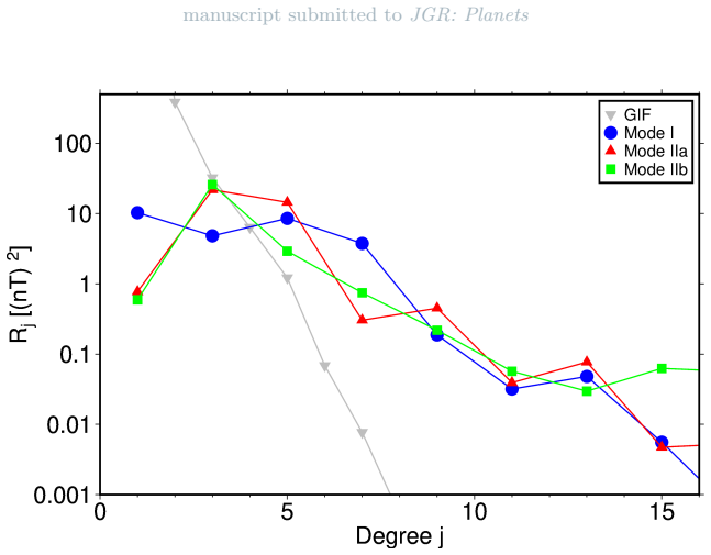
Under the reference interior model, with ocean thickness 361 km, ice shell 70 km, and ocean conductivity 5 S/m, the stationary ocean-induced magnetic field, produced mainly by the toroidal zonal-jet component of the flow interacting with Ganymede's internal dipole field, reaches 5.2–5.8 nT in the radial component at the surface. This signal exceeds the extrapolated core-field power at spherical-harmonic degrees 5 and above, giving a spectral window in which the ocean's motion dominates. The spatial pattern identifies the flow regime: Mode IIa reverses the signs of the key features relative to Modes I and IIb, and Mode I versus Mode IIb can be separated by local extrema in the zonally averaged field. For Mode IIa, the equatorial peak of the zonally averaged radial field shifts from 54.7 to 40.8 to 34.8 degrees latitude as the radius ratio ri/ro goes from 0.80 to 0.85 to 0.90, providing an ocean-thickness diagnostic once the ice thickness is known from other measurements.
Load-bearing premise
The whole measurability claim rests on the reference ocean conductivity of 5 S/m, which the authors themselves call a probable upper limit; the surface signal scales almost linearly with this value and would fall below detectability if the conductivity is an order of magnitude smaller.
Editorial extensions
If this is right
- If Juice or Europa Clipper detect the predicted pattern, the measured OIMF could identify Ganymede's convective regime among the three modeled flow modes.
- Ocean thickness can be estimated from the latitudinal position of the OIMF's equatorial peak once ice thickness is known, with Mode IIa giving the cleanest separation.
- The stationary OIMF adds magnetic power at spherical-harmonic degrees 5 and above, so spectral analysis can separate it from the predominantly dipolar core field.
- Because OIMF strength scales almost linearly with ocean conductivity, a detected or absent few-nT signal would discriminate between high-conductivity and low-conductivity ocean models.
- For thin oceans or thick ice shells the predicted signal falls below a few nT, so nondetection constrains ocean thickness and conductivity combinations rather than ruling out flow induction entirely.
Reading between the lines
- A natural next step is a synthetic retrieval study that puts this surface field through realistic Juice and Europa Clipper flyby trajectories and magnetometer noise models, testing whether the few-nT pattern and peak latitudes survive inversion.
- The same toroidal-flow-plus-dipole-ambient mechanism should apply to any ocean world with a strong internal field and sufficiently thick conductive ocean, so the method has a template extension beyond Ganymede.
- If independent tidal or libration data fix the ice thickness, a nondetection of the predicted OIMF pattern would push the ocean conductivity below roughly 0.5 S/m, turning the magnetometer into a compositional constraint on the ocean's salt content.
Editorial analysis
A structured set of objections, weighed in public.
Referee Report
Summary. This paper presents forward calculations of the magnetic field induced by convective flow (OIMF) in Ganymede's subsurface ocean. The authors solve the electromagnetic induction equation in a simplified form for a spherically symmetric, layered interior, using velocity fields from the companion manuscript Kvorka et al. (2025) and ambient fields from Connerney et al. (2022) and Weber et al. (2022). They find that, under a reference interior (ocean thickness 361 km, ice thickness 70 km, ocean conductivity 5 S/m), the stationary OIMF reaches 5.2–5.8 nT at the surface, is dominated by toroidal zonal jets interacting with Ganymede's internal dipole field, and has distinguishable spatial patterns for the three proposed flow modes. They further propose that the latitudinal position of the equatorial peak in the zonally averaged radial OIMF can be used to infer ocean thickness, with peak positions 54.7°, 40.8°, and 34.8° for ri/ro = 0.80, 0.85, and 0.90 in Mode IIa. The paper also includes a sensitivity study over ocean/ice thickness and conductivity and compares the simplified EMI solution with a fuller solution.
Significance. The study addresses a timely and important question: whether the upcoming JUICE and Europa Clipper magnetometer measurements can constrain the dynamics and structure of Ganymede's subsurface ocean. If the results hold, the OIMF would provide a new observable for ocean flow regime and thickness, extending the authors' earlier work on Europa. The forward EMI solver is a standard and tested approach, the decomposition of the OIMF into toroidal- and poloidal-flow contributions is conceptually clear, and the sensitivity study is transparent, with the authors explicitly acknowledging the upper-limit nature of the reference ocean conductivity. However, the significance of the quantitative claims is currently limited by the fact that the flow patterns, mode taxonomy, and 'most probable Mode IIb' selection are taken from a same-group manuscript that is not yet available, and by the lack of a quantitative validation of the simplified EMI equation. The paper's central predictions are falsifiable and well formulated, but they are not yet independently checkable from the manuscript alone.
major comments (4)
- [Section 3 (and Figures 1, 5, 9)] All quantitative results—the 5.2–5.8 nT amplitudes, the Mode IIa sign reversal, and the ocean-thickness diagnostic with equatorial peaks at 54.7°, 40.8°, and 34.8°—are computed with velocity fields from Kvorka et al. (2025), a same-group manuscript that is only 'submitted to Icarus' and not available to the reader. Because the OIMF is a linear functional of the flow, its spatial structure is entirely set by the jet latitudes, widths, and speeds of those convection simulations. No sensitivity run is presented in which the jet profile is perturbed, so the paper cannot currently rule out that the proposed mode identification and thickness diagnostic are artifacts of a particular convection simulation. Please provide the essential details of the Kvorka et al. model (parameter values, resolution, boundary conditions, and the extrapolation method used to obtain speeds at Q = 1 TW and D = 361 km) or a synthetic-perturbation analysis that demonstrates robustness of the OIMF pattern.
- [Section 6.1 / Supplementary material] The validation of the Simplified solution against the Full solution is qualitative: the text reports that 'differences are relatively subtle' and that 'large-scale patterns are the same,' while the Supplementary material asserts that neglecting the ocean-induced field in the advection term is 'likely below 10%' without showing that calculation. Since the Simplified approach is used for all subsequent results, including the thickness diagnostic, the paper should report a quantitative misfit metric (e.g., degree-by-degree relative power or RMS difference of the radial component) for the reference case and for the parameter variations in Section 6.4.
- [Sections 6.4 and 7] The measurability claim is strongly dependent on the assumed ocean conductivity: Figure 7a shows an almost linear scaling, and the authors state in Section 5 that the reference σ_o = 5 S/m 'probably represents the corresponding upper limit' and in Section 7 that an order-of-magnitude smaller conductivity, as suggested by Jia et al. (2025) and Saur et al. (2015), would make the OIMF undetectable. This caveat is transparent, but the abstract and key points nevertheless present the few-nT value as the headline result. To make the measurability claim quantitatively meaningful, the paper should compare the OIMF amplitude with the actual noise and measurement geometry of the JUICE and Europa Clipper magnetometers at Ganymede, rather than only citing instrument sensitivity limits.
- [Section 6.5] The proposed ocean-thickness diagnostic relies on resolving shifts in the latitudinal position of the equatorial peak of the zonally averaged |Br|. For Mode IIa the peak shifts are 13.9° and 6.0° between ri/ro = 0.80/0.85/0.90, but for Mode I they are only 4.0° and 1.9°, and for Mode IIb 4.0° and 2.0°; the authors acknowledge that 0.85 versus 0.90 'could be difficult to distinguish' in these modes. The paper should estimate the along-track sampling and noise level required to resolve such peak shifts, and should discuss how misidentification of the flow mode (e.g., Mode I vs IIa) would propagate into the thickness inference.
minor comments (6)
- [Section 6.4, Figure 7a text] The sentence 'the OIMF increases from 1.7 S/m to 5.2 S/m and 10.4 S/m' should read '1.7 nT to 5.2 nT and 10.4 nT'.
- [Section 3] The phrase 'using the extrapolation method proposed by Kvorka et al. (2025)' is not self-contained; a one-sentence summary of the method would help the reader assess the uncertainty in the flow speeds.
- [Section 6.1] The comparison of Configuration 1 with the Europa results of Sachl et al. (2025) is qualitative; please provide a table of the parameter differences (size, ocean thickness, JMF amplitude, flow speed) mentioned in the text.
- [Section 6.3] The statement that 'the true decrease of the GIF spectrum may be steeper, as the power spectrum in Christensen (2015a) was calculated using the defective code' is vague; please specify how the corrected spectrum (Christensen, 2015b) changes R2/R1 and whether the OIMF/GIF crossover at degree 5 is affected.
- [Section 6.5] Please define 'peak closest to the equator' more explicitly for the zonally averaged |Br| profiles, especially when the profile has multiple local maxima (e.g., Mode I in Figure 8).
- [Open Research Section] The data availability statement is incomplete: 'Modeling results can be downloaded from' is followed by no repository link or contact information.
Circularity Check
Central claims inherit the unvalidated flow-mode taxonomy and speeds from a same-group submitted manuscript; the OIMF 'diagnostics' are linear images of those input flows, though the EMI solution itself is independent.
-
self citation load bearing
[Section 1 ('In the present study...'), Section 3, and the opening of Section 6 ('Mode IIb... most probable flow mode (Kvorka et al., 2025)')]
"In the present study, we use the models of Ganymede's ocean circulation developed by Kvorka et al. (2025) to investigate the OIMF ... The OIMFs presented in Sections 6.1 and 6.2 are calculated using Mode IIb, which is the most probable flow mode in Ganymede's ocean (Kvorka et al., 2025)."
All quantitative results — the 5.2–5.8 nT amplitudes, the mode-discriminating sign reversal, and the ocean-thickness diagnostic (peak latitudes 54.7°, 40.8°, 34.8° for ri/ro = 0.80, 0.85, 0.90) — are computed from velocity fields, flow modes, and speed scalings supplied by Kvorka et al. (2025), a same-group manuscript listed as 'submitted to Icarus' with placeholder 'xxx'. The OIMF is a linear functional of these flows (Eq. 17), so the spatial pattern and its ri/ro dependence are imposed by the input jets and their assumed tangent-cylinder geometry; the paper itself states that the shift 'stands to reason' from the flow geometry.
full rationale
The magnetic part of the derivation is self-contained: the paper solves the quasi-static EMI equation (Eq. 17) with standard linearizations, and it tests the Simplified treatment against the Full solution in Section 6.1 and against externally sourced ambient-field models (Connerney et al. 2022; Weber et al. 2022). No parameter is fitted to the predicted OIMF, and no predicted quantity is defined in terms of itself, so the core electromagnetic forward model is not circular. However, the paper's scientific claims about what the OIMF can measure are conditional on the flow fields, modes, and speeds from Kvorka et al. (2025), a same-group submitted manuscript that is unavailable to the reader. Because the OIMF pattern is essentially the zonal-jet structure of those flows mapped through a linear PDE, the mode-identification and ocean-thickness diagnostics inherit the assumptions of the self-cited flow simulation without an independent validation or a sensitivity run in which the flow is perturbed. The paper does openly flag the conductivity uncertainty as an upper limit (Section 5) and notes the non-detectability at lower conductivity (Section 7), which is a genuine caveat. Overall, this is a load-bearing self-citation with the central EM derivation retaining independent content, giving a circularity score of 4.
Assumptions & free parameters
free parameters (5)
- reference ocean electrical conductivity sigma_o =
5 S/m
- reference ocean thickness D =
361 km; ri/ro 0.80 to 0.95 maps to 513 to 128 km at H=70 km
- reference ice shell thickness H =
70 km
- interior heat flow Q used to set flow speeds =
1 TW reference; 200 to 1600 GW range
- flow mode used for the main calculations =
Mode IIb (most probable per Kvorka et al. 2025)
assumptions (6)
- standard math Quasi-static Maxwell equations and Ohm's law in a moving continuum
- domain assumption The core dynamo field BC is a stationary potential field
- domain assumption The ocean-induced field can be neglected in the advection term, with error below 10 percent
- domain assumption Motionless induction can be neglected and Jupiter's field treated as potential inside Ganymede
- domain assumption Spherically symmetric 1-D conductivity structure
- domain assumption The same-group convection simulations of Kvorka et al. (2025) represent the true ocean circulation and its flow modes
Cite this review
Pith. "Pith review of Can the magnetic field induced by convective flow constrain the properties of Ganymede's subsurface ocean?." pith.science (2026). https://pith.science/paper/PQOYQ6OJ
@misc{pith2026250708576,
  author       = {Pith},
  title        = {Pith review of: Can the magnetic field induced by convective flow constrain the properties of Ganymede's subsurface ocean?},
  year         = {2026},
  howpublished = {\url{https://pith.science/paper/PQOYQ6OJ}},
  note         = {Machine review of arXiv:2507.08576}
}
read the original abstract
This paper has two main objectives. First, we assess the strength and measurability of Ganymede's ocean-induced magnetic field (OIMF) generated by the flow in the subsurface ocean. Second, we inspect how the OIMF constrains the ocean flow and Ganymede's internal structure and suggest a suitable metric for this purpose. We calculate the OIMF by solving the electromagnetic induction (EMI) equation in the simplified form, where we neglect the ocean-induced field in the advection term and the motionless induction. We show that this approach is sufficiently accurate by comparison with the solution of the full EMI equation. We also demonstrate that the OIMF is predominantly a stationary signal generated by the interaction of the toroidal component of the flow with Ganymede's internal field. The contributions to the OIMF due to the poloidal component of the flow and Jupiter's magnetic field can be neglected as second-order effects. The stationary OIMF is a measurable quantity with a few nT amplitude on Ganymede's surface if the ocean is sufficiently thick (approximately 400 km) and conductive (approximately 5 S/m). In this case, the specific footprint of the measured OIMF could be used to identify the flow regime (mode) of the convecting ocean. Additionally, the OIMF can be used to determine the ocean thickness since the OIMF pattern is shifted towards low latitudes if the ocean thickness is reduced.
Figures


Figures from the paper (6 more)




Reference graph
Works this paper leans on
-
[1]
amit2020 APACrefauthors Amit, H. , Choblet, G. , Tobie, G. , Terra-Nova, F. , Čadek, O. \ Bouffard, M. APACrefauthors \ 2020 . Cooling patterns in rotating thin spherical shells -- Application to Titan's subsurface ocean Cooling patterns in rotating thin spherical shells -- Application to Titan's subsurface ocean . Icarus 338 113509 . APACrefDOI doi:10.10...
-
[2]
Andersson2005 APACrefauthors Andersson, O. \ Inaba, A. APACrefauthors \ 2005 . Thermal conductivity of crystalline and amorphous ices and its implications on amorphization and glassy water Thermal conductivity of crystalline and amorphous ices and its implications on amorphization and glassy water . Physical Chemistry Chemical Physics 7 7 1441--1449
work page 2005
-
[3]
ashkenazy2021 APACrefauthors Ashkenazy, Y. \ Tziperman, E. APACrefauthors \ 2021 . Dynamic E uropa ocean shows transient T aylor columns and convection driven by ice melting and salinity Dynamic E uropa ocean shows transient T aylor columns and convection driven by ice melting and salinity . Nature Communications 12 6376 . APACrefDOI doi:10.1038/s41467-02...
-
[4]
ashkenazy2022 APACrefauthors Ashkenazy, Y. , Tziperman, E. \ Nimmo, F. APACrefauthors \ 2023 . Non-synchronous rotation on Europa driven by ocean currents Non-synchronous rotation on Europa driven by ocean currents . AGU Advances 4 e2022AV000849 . APACrefDOI doi:10.1029/2022AV000849 APACrefDOI
-
[5]
bire2022 APACrefauthors Bire, S. , Kang, W. , Ramadhan, A. , Campin, J M. \ Marshall, J. APACrefauthors \ 2022 . Exploring ocean circulation on icy moons heated from below Exploring ocean circulation on icy moons heated from below . Journal of Geophysical Research: Planets 127 e2021JE007025 . APACrefDOI doi:10.1029/2021JE007025 APACrefDOI
-
[6]
bire2023 APACrefauthors Bire, S. , Mittal, T. , Kang, W. , Ramadhan, A. , Tuckman, P J. , German, C R. Marshall, J. APACrefauthors \ 2023 . Divergent Behavior of Hydrothermal Plumes in Fresh Versus Salty Icy Ocean Worlds Divergent behavior of hydrothermal plumes in fresh versus salty icy ocean worlds . Journal of Geophysical Research: Planets 128 e2023JE0...
-
[7]
Bland2008 APACrefauthors Bland, M T. , Showman, A P. \ Tobie, G. APACrefauthors \ 2008 . The production of G anymede's magnetic field The production of G anymede's magnetic field . Icarus 198 2 384--399 . APACrefDOI doi:10.1016/j.icarus.2008.07.011 APACrefDOI
-
[8]
cabanes2024 APACrefauthors Cabanes, S. , Gastine, T. \ Fournier, A. APACrefauthors \ 2024 . Zonostrophic turbulence in the subsurface oceans of the Jovian and Saturnian moons Zonostrophic turbulence in the subsurface oceans of the Jovian and Saturnian moons . Icarus 415 116047 . APACrefDOI doi:10.1016/j.icarus.2024.116047 APACrefDOI
Show all 59 references
-
[9]
, Aurnou, J M
cheng2018 APACrefauthors Cheng, J S. , Aurnou, J M. , Julien, K. \ Kunnen, R P J. APACrefauthors \ 2018 . A heuristic framework for next-generation models of geostrophic convective turbulence A heuristic framework for next-generation models of geostrophic convective turbulence...
2018
-
[10]
, Tobie, G
choblet2017 APACrefauthors Choblet, G. , Tobie, G. , Sotin, C. , Kalousov \' a , K. \ Grasset, O. APACrefauthors \ 2017 . Heat transport in the high-pressure ice mantle of large icy moons Heat transport in the high-pressure ice mantle of large icy moons . Icarus 285 252-262 . ...
2017 doi
-
[12]
APACrefauthors \ 2015 2
Christensen2015b APACrefauthors Christensen , U R. APACrefauthors \ 2015 2 . Iron snow dynamo models for G anymede (vol 247, pg 248, 2015) Iron snow dynamo models for G anymede (vol 247, pg 248, 2015) . Icarus 256 63-65 . APACrefDOI doi:10.1016/j.icarus.2015.04.022 APACrefDOI
2015 doi
-
[13]
, Timmins, S
Connerney2022 APACrefauthors Connerney, J E P. , Timmins, S. , Oliversen, R J. , Espley, J R. , Joergensen, J L. , Kotsiaros, S. others APACrefauthors \ 2022 . A new model of Jupiter 's magnetic field at the completion of Juno 's Prime Mission A new model of Jupiter 's magneti...
2022 doi
-
[14]
, Betzler , A
ellmaier2024 APACrefauthors Ellmeier , M. , Betzler , A. , Amtmann , C. , Pollinger , A. , Hagen , C. , Jernej , I. Lammegger , R. APACrefauthors \ 2024 . Lower magnetic field measurement limit of the coupled dark state magnetometer Lower magnetic field measurement limit of th...
2024 doi
-
[15]
, Velímský , J
Finlay2024 APACrefauthors Finlay , C. , Velímský , J. , C., K. \ Blangsbøll , R. APACrefauthors \ 2024 . Satellite monitoring of long period ocean-induced magnetic field variations Satellite monitoring of long period ocean-induced magnetic field variations . PTRS 382 20240077 ...
2024
-
[16]
, Wicht, J
gastine2016 APACrefauthors Gastine, T. , Wicht, J. \ Aubert, J. APACrefauthors \ 2016 . Scaling regimes in spherical shell rotating convection Scaling regimes in spherical shell rotating convection . Journal of Fluid Mechanics 808 690–732 . APACrefDOI doi:10.1017/jfm.2016.659 ...
2016 doi
-
[17]
, Finlay, C C
Grayver2024 APACrefauthors Grayver, A. , Finlay, C C. \ Olsen, N. APACrefauthors \ 2024 . Magnetic signals from oceanic tides: new satellite observations and applications Magnetic signals from oceanic tides: new satellite observations and applications . PTRS 382 20240078 . APA...
2024
-
[18]
, Munch, F D
Grayver2017 APACrefauthors Grayver , A V. , Munch, F D. , Kuvshinov, A V. , Khan, A. , Kuvshinov2006, T J. \ T ffner-Clausen, L. APACrefauthors \ 2017 . Joint inversion of satellite-detected tidal and magnetospheric signals constrains electrical conductivity and water content ...
2017
-
[19]
\ Olsen, N
Grayver2019 APACrefauthors Grayver , A V. \ Olsen, N. APACrefauthors \ 2019 . The magnetic signatures of the M2 , N2 , and O1 oceanic tides observed in Swarm and CHAMP satellite magnetic data The magnetic signatures of the M2 , N2 , and O1 oceanic tides observed in Swarm and C...
2019 doi
-
[20]
, Kurth, W S
gurnett1996 APACrefauthors Gurnett, D A. , Kurth, W S. , Roux, A. , Bolton, S J. \ Kennel, C F. APACrefauthors \ 1996 . Evidence for a magnetosphere at G anymede from plasma-wave observations by the G alileo spacecraft Evidence for a magnetosphere at G anymede from plasma-wave...
1996 doi
-
[21]
\ Chyba, C F
Hand2007 APACrefauthors Hand, K P. \ Chyba, C F. APACrefauthors \ 2007 . Empirical constraints on the salinity of the europan ocean and implications for a thin ice shell Empirical constraints on the salinity of the europan ocean and implications for a thin ice shell . Icarus 1...
2007 doi
-
[22]
, Aurnou , J M
Hauck2006 APACrefauthors Hauck II , S A. , Aurnou , J M. \ Dombard , A J. APACrefauthors \ 2006 . Sulfur's impact on core evolution and magnetic field generation on Ganymede Sulfur's impact on core evolution and magnetic field generation on Ganymede . Journal of Geophysical Re...
2006 doi
-
[23]
, Kivelson, M G
Jia2025 APACrefauthors Jia, X. , Kivelson, M G. , Khurana, K K. \ Walker, R J. APACrefauthors \ 2025 . Improved models of Ganymede 's permanent and induced magnetic fields based on Galileo and Juno data Improved models of Ganymede 's permanent and induced magnetic fields based...
2025
-
[24]
, Bire , S
kang2022a APACrefauthors Kang , W. , Bire , S. \ Marshall , J. APACrefauthors \ 2022a . The role of ocean circulation in driving hemispheric symmetry breaking of the ice shell of Enceladus The role of ocean circulation in driving hemispheric symmetry breaking of the ice shell ...
-
[25]
, Mittal , T
kang2022b APACrefauthors Kang , W. , Mittal , T. , Bire , S. , Campin , S M. \ Marshall , J. APACrefauthors \ 2022b . How does salinity shape ocean circulation and ice geometry on Enceladus and other icy satellites? How does salinity shape ocean circulation and ice geometry on...
-
[26]
\ Frischknecht, F C
Keller1966 APACrefauthors Keller, G V. \ Frischknecht, F C. APACrefauthors \ 1966 . Electrical methods in geophysical prospecting Electrical methods in geophysical prospecting . Pergamon Press, Oxford
1966
-
[27]
, Jia, X
Kivelson2023 APACrefauthors Kivelson, M G. , Jia, X. , Lee, K A. , Raymond, C A. , Khurana, K K. , Perley, M O. others APACrefauthors \ 2023 . The Europa Clipper Magnetometer The Europa Clipper Magnetometer . Space Science Reviews 219 6 48 . APACrefDOI doi:10.1007/s11214-023-0...
2023 doi
-
[28]
, Khurana, K K
kivelson1997a APACrefauthors Kivelson, M G. , Khurana, K K. , Coroniti, F V. , Joy, S. , Russell, C T. , Walker, R J. Polanskey, C. APACrefauthors \ 1997 . The magnetic field and magnetosphere of G anymede The magnetic field and magnetosphere of G anymede . Geophysical Researc...
1997 doi
-
[29]
, Khurana, K K
kivelson1996 APACrefauthors Kivelson, M G. , Khurana, K K. , Russell, C T. , Walker, R J. , Warnecke, J. , Coroniti, F V. Schubert, G. APACrefauthors \ 1996 . Discovery of G anymede's magnetic field by the G alileo spacecraft Discovery of G anymede's magnetic field by the G al...
1996 doi
-
[30]
, Khurana, K K
Kivelson2002 APACrefauthors Kivelson, M G. , Khurana, K K. \ Volwerk, M. APACrefauthors \ 2002 . The permanent and inductive magnetic moments of Ganymede The permanent and inductive magnetic moments of Ganymede . Icarus 157 2 507--522 . APACrefDOI doi:10.1006/icar.2002.6834 APACrefDOI
2002
-
[31]
\ Kronrod, V A
Kuskov2001 APACrefauthors Kuskov, O L. \ Kronrod, V A. APACrefauthors \ 2001 . Core sizes and internal structure of E arth's and J upiter's satellites Core sizes and internal structure of E arth's and J upiter's satellites . Icarus 151 2 204--227 . APACrefDOI doi:10.1006/icar....
2001
-
[32]
\ Čadek, O
kvorka2022 APACrefauthors Kvorka, J. \ Čadek, O. APACrefauthors \ 2022 . A numerical model of convective heat transfer in Titan’s subsurface ocean A numerical model of convective heat transfer in Titan’s subsurface ocean . Icarus 376 114853 . APACrefDOI doi:10.1016/j.icarus.20...
2022
-
[33]
\ Čadek, O
kvorka2024 APACrefauthors Kvorka, J. \ Čadek, O. APACrefauthors \ 2024 . The role of subsurface ocean dynamics and phase transitions in forming the topography of icy moons The role of subsurface ocean dynamics and phase transitions in forming the topography of icy moons . Icar...
2024
-
[34]
, C adek, O
kvorka2025 APACrefauthors Kvorka, J. , C adek, O. , S achl , L. \ Vel\' i msk\' y , J. APACrefauthors \ 2025 . xxx xxx . submitted to Icarus
2025
-
[35]
\ Sanford, T B
Larsen85 APACrefauthors Larsen, J C. \ Sanford, T B. APACrefauthors \ 1985 . Florida Current volume transports from voltage measurements Florida current volume transports from voltage measurements . Science 227 4684 302--304 . APACrefDOI doi:10.1126/science.227.4684.302 APACrefDOI
1985 doi
-
[36]
, Bierson, C J
lemasquerier2023 APACrefauthors Lemasquerier, D G. , Bierson, C J. \ Soderlund, K M. APACrefauthors \ 2023 . Europa's ocean translates interior tidal heating patterns to the ice-ocean boundary Europa's ocean translates interior tidal heating patterns to the ice-ocean boundary ...
2023 doi
-
[37]
, Kuvshinov, A
Manoj2006 APACrefauthors Manoj, C. , Kuvshinov, A. , Maus, S. \ L \"u hr, H. APACrefauthors \ 2006 . Ocean circulation generated magnetic signals Ocean circulation generated magnetic signals . Earth, Planets and Space 58 4 429--437 . APACrefDOI doi:10.1186/BF03351939 APACrefDOI
2006 doi
-
[38]
, Fullea, J
Martinec2021 APACrefauthors Martinec, Z. , Fullea, J. , Vel \' msk \'y , J. \ S achl, L. APACrefauthors \ 2021 . A new integrated geophysical-petrological global 3-D model of upper-mantle electrical conductivity validated by the Swarm M 2 tidal magnetic field A new integrated ...
2021
-
[39]
, Vance, S
Marusiak2021 APACrefauthors Marusiak, A G. , Vance, S. , Panning, M P. , B e hounkov \'a , M. , Byrne, P K. , Choblet, G. others APACrefauthors \ 2021 . Exploration of icy ocean worlds using geophysical approaches Exploration of icy ocean worlds using geophysical approaches . ...
2021 doi
-
[40]
, Yong, W
Pan2020 APACrefauthors Pan, Y. , Yong, W. \ Secco, R A. APACrefauthors \ 2020 . Electrical conductivity of aqueous magnesium sulfate at high pressure and low temperature with application to Ganymede's subsurface ocean Electrical conductivity of aqueous magnesium sulfate at hig...
2020
-
[41]
, T ffner-Clausen, L
Sabaka2020 APACrefauthors Sabaka, T J. , T ffner-Clausen, L. , Olsen, N. \ Finlay, C C. APACrefauthors \ 2020 . CM6 : a comprehensive geomagnetic field model derived from both CHAMP and S warm satellite observations CM6 : a comprehensive geomagnetic field model derived from bo...
2020 doi
-
[42]
, Knopp, O
Sachl2024 APACrefauthors S achl, L. , Knopp, O. \ Vel \' msk \'y , J. APACrefauthors \ 2024 . Electrical conductivity of the suboceanic upper mantle constrained by satellite-derived tidal magnetic fields: 3-D inversion, validation and interpretation Electrical conductivity of ...
2024 doi
-
[43]
, Martinec, Z
Sachl2019 APACrefauthors S achl, L. , Martinec, Z. , Vel \' msk \' y , J. , Irrgang, C. , Petereit, J. , Saynisch, J. Schnepf, N R. APACrefauthors \ 2019 . Modelling of electromagnetic signatures of global ocean circulation: physical approximations and numerical issues Modelli...
2019 doi
-
[44]
, Vel \' msk \'y , J
Sachl2022 APACrefauthors S achl, L. , Vel \' msk \'y , J. , Fullea, J. \ Martinec, Z. APACrefauthors \ 2022 . Inversion of the satellite observations of the tidally induced magnetic field in terms of 3-D upper-mantle electrical conductivity: method and synthetic tests Inversio...
2022
-
[45]
APACrefauthors \ 1971
Sanford71 APACrefauthors Sanford, T B. APACrefauthors \ 1971 . Motionally induced electric and magnetic fields in the sea Motionally induced electric and magnetic fields in the sea . Journal of Geophysical Research 76 15 3476--3492 . APACrefDOI doi:10.1029/JC076i015p03476 APACrefDOI
1971 doi
-
[46]
, Duling, S
Saur2015 APACrefauthors Saur, J. , Duling, S. , Roth, L. , Jia, X. , Strobel, D F. , Feldman, P D. others APACrefauthors \ 2015 . The search for a subsurface ocean in Ganymede with Hubble Space Telescope observations of its auroral ovals The search for a subsurface ocean in Ga...
2015
-
[47]
, Schmidt, B
soderlund2014 APACrefauthors Soderlund, K. , Schmidt, B. \ Wicht, J. APACrefauthors \ 2014 . Ocean-driven heating of Europa’s icy shell at low latitudes Ocean-driven heating of Europa’s icy shell at low latitudes . Nature Geoscience 7 16–19 . APACrefDOI doi:10.1038/ngeo2021 APACrefDOI
2014 doi
-
[48]
APACrefauthors \ 2019
soderlund2019 APACrefauthors Soderlund , K M. APACrefauthors \ 2019 . Ocean dynamics of outer solar system satellites Ocean dynamics of outer solar system satellites . Geophysical Research Letters 46 8700-8710 . APACrefDOI doi:10.1029/2018GL081880 APACrefDOI
2019 doi
-
[49]
, Amit, H
terranova2023 APACrefauthors Terra-Nova, F. , Amit, H. , Choblet, G. , Tobie, G. , Bouffard, M. \ Čadek, O. APACrefauthors \ 2023 . The influence of heterogeneous seafloor heat flux on the cooling patterns of Ganymede’s and Titan’s subsurface oceans The influence of heterogene...
2023
-
[50]
, Maus, S
Tyler2003 APACrefauthors Tyler, R H. , Maus, S. \ Luhr, H. APACrefauthors \ 2003 . Satellite observations of magnetic fields due to ocean tidal flow Satellite observations of magnetic fields due to ocean tidal flow . Science 299 5604 239--241 . APACrefDOI doi:10.1126/science.1...
2003 doi
-
[51]
, Panning, M P
vance2018 APACrefauthors Vance, S D. , Panning, M P. , Stähler, S. , Cammarano, F. , Bills, B G. , Tobie, G. Banerdt, B. APACrefauthors \ 2018 . Geophysical investigations of habitability in ice-covered ocean worlds Geophysical investigations of habitability in ice-covered oce...
2018 doi
-
[52]
, Styczinski, M J
vance2021 APACrefauthors Vance, S D. , Styczinski, M J. , Bills, B G. , Cochrane, C J. , Soderlund, K M. , Gómez-Pérez, N. \ Paty, C. APACrefauthors \ 2021 . Magnetic induction responses of Jupiter's ocean moons including effects from adiabatic convection Magnetic induction re...
2021 doi
-
[53]
, Grayver, A
Velimsky2018 APACrefauthors Vel \' msk \'y , J. , Grayver, A. , Kuvshinov, A. \ S achl, L. APACrefauthors \ 2018 . On the modelling of M 2 tidal magnetic signatures: Effects of physical approximation and numerical resolution On the modelling of M 2 tidal magnetic signatures: E...
2018 doi
-
[54]
, Schnepf , N
Velimsky2021b APACrefauthors Velímský , J. , Schnepf , N. , Nair , M. \ Thomas , N. APACrefauthors \ 2021 . Can seafloor voltage cables be used to study large-scale circulation? A n investigation in the P acific O cean Can seafloor voltage cables be used to study large-scale c...
2021 doi
-
[55]
, Maier-Reimer, E
Vivier2004 APACrefauthors Vivier, F. , Maier-Reimer, E. \ Tyler, R H. APACrefauthors \ 2004 . Simulations of magnetic fields generated by the A ntarctic C ircumpolar C urrent at satellite altitude: C an geomagnetic measurements be used to monitor the flow? Simulations of magne...
2004 doi
-
[56]
, Kvorka , J
Sachl2025 APACrefauthors S achl , L. , Kvorka , J. , C adek , O. \ Velímský , J. APACrefauthors \ 2025 . Magnetic field induced by convective flow in E uropa’s subsurface ocean Magnetic field induced by convective flow in E uropa’s subsurface ocean . Icarus 429 116375 . APACre...
2025
-
[57]
, Moore, K
Weber2022 APACrefauthors Weber, T. , Moore, K. , Connerney, J. , Espley, J. , DiBraccio, G. \ Romanelli, N. APACrefauthors \ 2022 . Updated spherical harmonic magnetic field moments of G anymede from the J uno flyby Updated spherical harmonic magnetic field moments of G anymed...
2022 doi
-
[58]
, Gastine, T
yadav2015 APACrefauthors Yadav, R K. , Gastine, T. , Christensen, U R. , Duarte, L D V. \ Reiners, A. APACrefauthors \ 2015 . Effect of shear and magnetic field on the heat-transfer efficiency of convection in rotating spherical shells Effect of shear and magnetic field on the...
2015 doi
-
[59]
, Khurana, K K
Zimmer2000 APACrefauthors Zimmer, C. , Khurana, K K. \ Kivelson, M G. APACrefauthors \ 2000 . Subsurface oceans on Europa and Callisto : Constraints from Galileo magnetometer observations Subsurface oceans on Europa and Callisto : Constraints from Galileo magnetometer observat...
2000
-
[60]
APACrefauthors \ 2015
Christensen2015a APACrefauthors Christensen , U R. APACrefauthors \ 2015 . Iron snow dynamo models for G anymede Iron snow dynamo models for G anymede . Icarus 247 248-259 . APACrefDOI doi:10.1016/j.icarus.2014.10.024 APACrefDOI
2015 doi
Reviewed August 6, 2026 · model on record in the stance chip above.
Discussion (0). Sign in to comment.