REVIEW 2 major objections 5 minor 2 cited by
Central limit theorems for the Euler characteristic in the Random Connection Model for higher-dimensional simplicial complexes
T0 review · 2 major / 5 minor · reviewed 2026-08-07 · deepseek-v4-flash
Pith's one-line read A generalized Euler characteristic of higher-dimensional random connection models is asymptotically normal in both high-intensity and large-window regimes, with explicit Wasserstein and Kolmogorov error rates.
desk verdict Solid new model and likely-correct CLTs; the large-window proof hinges on Lemma 6.5, whose most delicate bounds are still a sketch. read the letter →
The pith
A machine-rendered reading of the paper's core claim, the machinery that carries it, and where it could break.
The reading
What carries the argument
The argument runs on integral representations $I_K(W)=\int_{W^r} \prod_{\sigma\in K} \varphi_{|\sigma|-1}(x_\sigma)\,\lambda^r(d(x_1,\dots,x_r))$, which encode the probability weight of a fixed combinatorial simplicial complex $K$ appearing inside $\Delta_W$. The difference operators $\Lambda^k_{(x_1,U_1),\dots,(x_l,U_l)}$ are constructed so that, applied to the Euler characteristic, they simply count simplices containing all $k$ added points and none of the others; this makes products of such operators tractable. A Fock-space representation expresses the variance as a sum of nonnegative terms and yields the lower bound $\operatorname{Var}(\chi_a(\Delta_W))\ge a_\alpha^2 \beta^{\alpha+1} I^{\alpha+1}_{\alpha+1,\alpha+1}(W)/(\alpha+1)!$. The normal approximation comes from Poisson-space normal approximation bounds adapted to these modified operators, which replace the usual add-one operators. Condition (22) is the step that forces every connected integral representation to be at most $C|W|$, which is what turns all six error terms into order $|W|^{-1/2}$ after standardization.
What would settle it
Take $X=\mathbb{R}$ with Lebesgue intensity and $\varphi_1(x,y)=\min\{1,|x-y|^{-p}\}$ with $p<1/2$, so that $\int \varphi_1^{1/2}\,d\lambda=\infty$; then compute $\operatorname{Var}(\chi_a(\Delta_{[-n,n]}))$ as $n\to\infty$. Linear growth would mean condition (22) is stronger than needed; superlinear growth, or a non-normal limit under $\sqrt{n}$ scaling, would show the theorem has reached its natural boundary.
Extended reading notes
Core claim
The central claim is that the generalized Euler characteristic of the random connection model is asymptotically Gaussian in the regimes where the amount of randomness goes to infinity, either through the intensity or through the observation window. Concretely, Theorem 6.2 states that if $I^{\alpha+1}_{\alpha+1,\alpha+1}(W)>0$, then $(\chi_a(\Delta_W)-\mathbb{E}[\chi_a(\Delta_W)])/\sqrt{\operatorname{Var}(\chi_a(\Delta_W))}$ converges in distribution to $N(0,1)$ as $\beta\to\infty$, with the six error quantities of Theorem 5.1 satisfying $\gamma_1,\gamma_3,\gamma_4,\gamma_5=O(\beta^{-1/2})$, $\gamma_2=O(\beta^{-3/2})$, and $\gamma_6=O(\beta^{-1})$. Theorem 6.6 establishes the analogous result for sequences of windows with $|W_n|\to\infty$ under condition (22), $\nu=\sup_x \int_X \varphi_1(x,y)^{1/2}\lambda(dy)<\infty$, together with a linear lower bound on the expected number of top-dimensional simplices; in that regime all six error terms are $O(|W_n|^{-1/2})$. Theorem 7.3 derives a multivariate CLT for the simplex-count vector in the marked stationary case, with a positive definite limiting covariance matrix $\Sigma$. The underlying discovery is that, despite the complex dependence created by the simplex-formation rules, the generalized Euler characteristic has variance of order the expected number of top-dimensional simplices, and its fluctuations are normal with explicit rates.
Load-bearing premise
The entire growing-window theorem depends on the global bound $\nu=\sup_{x\in X}\int_X \varphi_1(x,y)^{1/2}\lambda(dy)<\infty$; if that constant is infinite, the estimates that force the variance to grow only linearly in $|W|$ break down, and the $\sqrt{|W|}$ normalization is no longer justified.
Editorial extensions
If this is right
- For a fixed window, the standardized generalized Euler characteristic is asymptotically normal as the intensity grows, with explicit Wasserstein and Kolmogorov error rates of order $\beta^{-1/2}$ and faster.
- For growing windows, condition (22) together with a linear lower bound on the expected top-simplex count yields a CLT with all six error bounds of order $|W_n|^{-1/2}$, so the $\sqrt{|W_n|}$ normalization is the right scaling.
- In the marked stationary case, the vector of simplex counts $(f_0(\Delta_W),\dots,f_\alpha(\Delta_W))$ satisfies a multivariate CLT with a positive definite limiting covariance matrix $\Sigma$.
- The classical Euler characteristic ($a_i=(-1)^i$) is included, and so are the Čech and Vietoris–Rips complexes as special connection-function choices.
- The variance lower bound is proportional to the expected number of top-dimensional simplices, so positivity of $I^{\alpha+1}_{\alpha+1,\alpha+1}$ is the non-degeneracy condition controlling the whole theorem.
Reading between the lines
- The exponent $1/2$ in condition (22) is forced by the smallest outside exponent appearing in the six error integrals, so relaxing the condition would likely require a different decomposition rather than a small tweak; this suggests the theorem is close to the natural limit of its method.
- A natural testable extension is to replace the supremum in (22) with an $L^p$-type average over $x$; the paper's method may still work when the averaged quantity is small, but this is not stated and would need a separate argument.
- Because the classical Euler characteristic is a special case, the CLTs imply that the signed simplex counts of Čech and Vietoris–Rips complexes fluctuate normally whenever the intensity or window growth makes the top-dimensional simplex count dominate the variance.
Signed reviews
Editorial analysis
A structured set of objections, weighed in public.
Referee Report
Summary. The paper introduces a higher-dimensional generalization of the random connection model: vertices are drawn from a Poisson process on a Borel space, and simplices of each dimension are added independently with probabilities given by symmetric connection functions. For the resulting random simplicial complex, the paper studies the generalized Euler characteristic with an arbitrary coefficient vector. It derives first- and second-moment formulas, a Fock-space-type variance representation, and quantitative normal approximation bounds based on a transfer theorem for Poisson functionals. The main results are a central limit theorem as the intensity β tends to infinity (Theorem 6.2), a central limit theorem as the observation window grows under the global integrability condition (22) and a lower-growth condition (36) (Theorem 6.6), and a multivariate central limit theorem for simplex counts in the marked stationary case (Theorem 7.3).
Significance. If the missing details are supplied, this is a substantial contribution. The model unifies several existing random simplicial complex constructions, the setting of an arbitrary Borel space is genuinely general, and the results come with explicit Wasserstein and Kolmogorov distance rates that are not tied to fitted parameters. The moment formulas in Section 4 and the operator transfer in Theorem 5.1 are carefully developed, and the proof of the β→∞ CLT is convincing. The paper also gives a transparent Fock-space lower bound for the variance and a clean combinatorial mechanism via connected integral representations in Lemma 6.4. The main unresolved point is the completeness of Lemma 6.5, on which the increasing-window CLT and the multivariate CLT rest.
major comments (2)
- [§6.2, Lemma 6.5] Lemma 6.5 is the load-bearing estimate for Theorem 6.6 and Theorem 7.3, but its proof is not complete as written. The proof details (24) and partially (23), then states that (25)–(29) can be established by the same method. The delicate point is that a naive bound such as f_i^{x_1,...,x_k} ≤ τ^{i+1-k} would give powers of |W| larger than 1; the required linear bound depends on expanding via the multivariate Mecke equation and using connectivity of the associated complexes together with condition (22). For (28), for example, one must show that the term E[(Λ²_{x_1,x_2}F)^4] produces a factor φ_1(x_1,x_2) that, after the outer exponent 1/2, lets the x_2-integral be controlled by ν from (22); without this cancellation one would obtain |W|² instead of |W|. Since the rates in Theorem 6.6 and the multivariate CLT in Theorem 7.3 depend directly on all six bounds, the proof should be completed for each of (25)–(29), or at least the reductions should be written out precisely enough that this cancellation is verifiable.
- [§6.2, proof of Lemma 6.5, display (23)] The proof of (23) is also written in a compressed way that makes it difficult to verify. The two expectations in (33) come from difference operators with different numbers of auxiliary points (l=2 and l=3), so the underlying complexes have different vertex sets; the intermediate notation f_L(x_1,…,x_{s+3}) is not defined for a complex L on s+2 vertices. Please rewrite the reduction with explicit vertex sets and relabelling, so that the final display (35) and the formation of the complex M in (34) are unambiguous.
minor comments (5)
- [Definition 4.1] In the displayed formula for κ_m, the product is over ∅≠I⊆{0,…,m+1}; it should be over ∅≠I⊆{0,…,m}, since κ_m is a function on X^{m+1}. The example for κ_2 in the following display confirms this.
- [§6.1, Lemma 6.1] The proof of Lemma 6.1 explicitly treats only the first displayed estimate; the remaining estimates are dismissed with 'this approach can easily be extended.' Since Theorem 6.2 uses all of them, please provide the short calculation or state the combinatorial bound that yields the claimed powers of β.
- [§6.2, proof of Lemma 6.5] The final remark that the outside exponents of the expectations in (23)–(29) lie in [1/2,1] is not literally correct for (25), (27), and the second summand of (28), where the outside exponent is 1; for exponent 1 the direct expansion used for (24) applies, so the remark should be rephrased.
- [§7, proof of Theorem 7.3] When Theorem 6.6 is applied to a coefficient vector whose top nonzero entry is b_s with s<α, the proof should explicitly say that the model is reduced to dimension s and that the higher-dimensional connection functions do not affect the functional; as written, the invocation of Theorem 6.6 is not literally covered by its statement, which assumes a_α≠0.
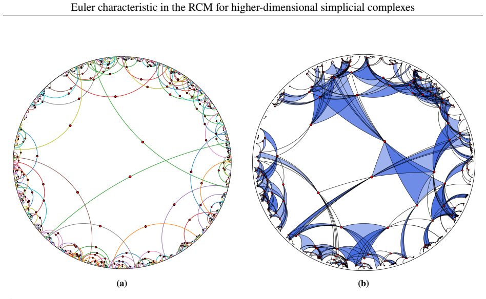
- [Throughout] There are several typographical slips, including 'allmost' and 'for allmost all n' in the proof of Theorem 6.6, an extraneous 'an' after 'F_n:=χ_a(Δ_{W_n})', 'connections functions' in the captions of Figures 1 and 2, and a missing parenthesis in the statement of Proposition 5.4.
Circularity Check
No circularity: central CLT proofs are derived from stated hypotheses and external normal-approximation theorems; self-citations are auxiliary and non-load-bearing.
full rationale
The derivation chain is self-contained with respect to its inputs. Theorem 5.1 adapts the external bounds of Last-Peccati-Schulte [13], and the paper supplies its own moment formulae (Proposition 4.3, Corollary 4.4), its own Fock-space variance representation (Proposition 5.4, including the lower bound (21)), and its own estimates for the resulting difference-operator terms (Lemmas 6.1, 6.4, 6.5). The non-degeneracy hypotheses, I^{alpha+1}_{alpha+1,alpha+1}(W)>0 for beta->infty and (36) for growing windows, are genuine assumptions and not restatements of the target CLT; they only guarantee that the variance grows at the required rate. No parameter is fitted and no predicted quantity equals an input by construction. The paper's only self-citations are to the author's PhD thesis [15]: once for an auxiliary fourth-moment computation that is explicitly bypassed via Lemma 4.2 of [13], and once for a technical Fock-space inequality that is instead recalculated in Proposition 5.4; neither is load-bearing. One caveat worth flagging is a completeness gap, not a circularity: Lemma 6.5 proves (24) and (23) in detail but dismisses (25)-(29) with 'in principle, this approach can be applied', so some decisive O(|W|) estimates rest on a sketch rather than a full proof. This affects rigor, not self-reference.
Assumptions & free parameters
assumptions (6)
- standard math Mecke's multivariate equation (Theorem 4.4 in [14])
- standard math Normal approximation bounds for Poisson functionals (Theorems 1.1 and 1.2 in [13])
- domain assumption Existence of a transitive measurable relation ≺ with λ([x]) = 0 for all x, extendable to arbitrary Borel spaces
- ad hoc to paper Global integrability condition (22): sup_x ∫ φ_1(x,y)^{1/2} λ(dy) < ∞
- ad hoc to paper Non-degeneracy condition I^{α+1}_{α+1,α+1}(W) > 0, or the growth condition (36) in the increasing-window setting
- standard math Cramér-Wold theorem and Slutsky's lemma
Cite this review
Pith. "Pith review of Central limit theorems for the Euler characteristic in the Random Connection Model for higher-dimensional simplicial complexes." pith.science (2026). https://pith.science/paper/PQPAYEZP
@misc{pith2026250611918,
  author       = {Pith},
  title        = {Pith review of: Central limit theorems for the Euler characteristic in the Random Connection Model for higher-dimensional simplicial complexes},
  year         = {2026},
  howpublished = {\url{https://pith.science/paper/PQPAYEZP}},
  note         = {Machine review of arXiv:2506.11918}
}
read the original abstract
As generalizations of random graphs, random simplicial complexes have been receiving growing attention in the literature. In this paper, we naturally extend the Random Connection Model (RCM), a random graph that has been extensively studied for over three decades, to a random simplicial complex, recovering many models currently found in the literature as special cases. In this new model, we derive quantitative central limit theorems for a generalized Euler characteristic in various asymptotic scenarios. We will accomplish this within a very general framework, where the vertices of the simplicial complex are drawn from an arbitrary Borel space.
Figures


Figures from the paper (1 more)

Forward citations
Cited by 2 Pith papers
-
Percolation in the marked stationary Random Connection Model for higher-dimensional simplicial complexes
A sharp phase transition for q-percolation is proven for the marked stationary random connection model on higher-dimensional simplicial complexes, unifying the Boolean, Vietoris-Rips, and Cech cases.
-
Betti numbers in the Random Connection Model for higher-dimensional simplicial complexes and the Boolean model
A central limit theorem is established for Betti numbers in the marked random connection model, and as a corollary for the Boolean model with general convex grains.
Reference graph
Works this paper leans on
-
[1]
A. Caicedo and M. Dickson. Critical Exponents for Marked Random Connection Models.Electronic Journal of Probability, 29(151):1–57, 2024. 2, 26
work page 2024
-
[2]
V. H. Can and K. D. Trinh. Random connection models in the thermodynamic regime: central limit theorems for add-one cost stabilizing functionals.Electronic Journal of Probability, 27(36):1–40, 2022. 2, 26
work page 2022
- [3]
-
[4]
A. Costa and M. Farber. Random Simplicial Complexes. In F. Callegaro, F. Cohen, C. De Concini, E. M. Feichtner, G. Gaiffi, and M. Salvetti, editors,Configuration Spaces: Geometry, Topology and Representation Theory, volume 14, pages 129–153. Springer, 2016. 2
work page 2016
-
[5]
M. Dickson and M. Heydenreich. The Triangle Condition for the Marked Random Connection Model. arXiv:2210.07727, 2022. 2, 26
arXiv 2022
-
[6]
Diestel.Graph Theory, volume 173 ofGraduate Texts in Mathematics
R. Diestel.Graph Theory, volume 173 ofGraduate Texts in Mathematics. Springer, fifth edition, 2017. 20, 27
work page 2017
-
[7]
C. Hirsch and D. Valesin. Face and cycle percolation.Journal of Applied and Computational Topology, 9(6):1–42, 2025. 2
work page 2025
-
[8]
D. Hug, G. Last, and M. Schulte. Second-order properties and central limit theorems for geometric functionals of Boolean models.The Annals of Applied Probability, 26(1):73–135, 2016. 27
work page 2016
Show all 22 references
-
[9]
M. Kahle. Topology of random clique complexes.Discrete Mathematics, 309(6):1658–1671, 2009. 2
2009
-
[10]
LimittheoremsforBettinumbersofrandomsimplicialcomplexes.Homology, Homotopy and Applications, 15(1):343–374, 2013
M.KahleandE.Meckes. LimittheoremsforBettinumbersofrandomsimplicialcomplexes.Homology, Homotopy and Applications, 15(1):343–374, 2013. 2
2013
-
[11]
Kallenberg.Foundations of Modern Probability, volume 99 ofProbability Theory and Stochastic Modelling
O. Kallenberg.Foundations of Modern Probability, volume 99 ofProbability Theory and Stochastic Modelling. Springer, third edition edition, 2021. 28
2021
-
[12]
Therandomconnectionmodelandfunctionsofedge-markedPois- son processes: Second order properties and normal approximation.The Annals of Applied Probability, 31(1):128–168, 2021
G.Last,F.Nestmann,andM.Schulte. Therandomconnectionmodelandfunctionsofedge-markedPois- son processes: Second order properties and normal approximation.The Annals of Applied Probability, 31(1):128–168, 2021. 2, 8, 11, 12, 13, 15, 26, 27
2021
-
[13]
NormalapproximationonPoissonspaces: Mehler’sformula,second order Poincaré inequalities and stabilization.Probability Theory and Related Fields, 165:667–723,
G.Last,G.Peccati,andM.Schulte. NormalapproximationonPoissonspaces: Mehler’sformula,second order Poincaré inequalities and stabilization.Probability Theory and Related Fields, 165:667–723,
-
[14]
Last and M
G. Last and M. D. Penrose.Lectures on the poisson process. Cambridge University Press, 2018. 5, 6, 8, 10, 12, 16, 23
2018
-
[15]
Pabst.Das Random Connection Model für höherdimensionale Simplizialkomplexe
D. Pabst.Das Random Connection Model für höherdimensionale Simplizialkomplexe. PhD thesis, Karlsruhe Institute of Technology, 2024. 4, 15, 16, 29
2024
-
[16]
M. Penrose. On a continuum percolation model.Advances in Applied Probability, 23(3):536–556,
-
[17]
Penrose.Random Geometric Graphs
M. Penrose.Random Geometric Graphs. Oxford studies in probability. Oxford University Press, 2003. 2
2003
-
[18]
J. G. Ratcliffe.Foundations of Hyperbolic Manifolds, volume 149 ofGraduate Texts in Mathematics. Springer, 3rd edition, 2019. 2
2019
-
[19]
Schneider and W
R. Schneider and W. Weil.Stochastic and integral geometry. Probability and Its Applications. Springer,
-
[20]
A. M. Thomas and T. Owada. Functional limit theorems for the Euler characteristic process in the critical regime.Advances in Applied Probability, 53:57–80, 2021. 4
2021
-
[21]
Yogeshwaran, E
D. Yogeshwaran, E. Subag, and R. J. Adler. Random geometric complexes in the thermodynamic regime.Probability Theory and Related Fields, 167:107–142, 2017. 2 30
2017
-
[2016]
4, 5, 11, 13, 14, 15
Reviewed August 7, 2026 · model on record in the stance chip above.
Discussion (0). Continue with ORCID to comment.