A Spline-based Physics-Informed Numerical Scheme: Accurate Smooth Solutions for Differential Equations
Pith reviewed 2026-05-20 02:33 UTC · model grok-4.3
The pith
A spline basis replaces neural networks to solve ODEs accurately while enforcing boundary conditions by construction.
A machine-rendered reading of the paper's core claim, the machinery that carries it, and where it could break.
Core claim
SPINS represents the unknown solution of an ODE by a spline basis chosen so that boundary conditions hold exactly, then minimizes the differential-equation residual with respect to the spline coefficients. Automatic differentiation supplies exact gradients of the residual, allowing rapid convergence under gradient-based optimizers. The resulting solution is a smooth, explicitly differentiable function whose accuracy is controlled by the spline degree and the number of knots.
What carries the argument
The structured spline basis (cubic or quintic interpolating splines) that encodes the trial solution and builds boundary conditions directly into the representation before any optimization occurs.
If this is right
- Boundary conditions are satisfied exactly rather than approximately through penalty terms.
- The solution remains a smooth, explicitly differentiable function at every stage of the computation.
- Optimization uses deterministic gradient methods and requires only a small number of coefficients.
- The framework extends directly to higher-order ODEs by raising the spline degree accordingly.
- Residual minimization becomes a standard nonlinear least-squares problem without stochastic sampling.
Where Pith is reading between the lines
- Multivariate spline bases could allow the same construction for certain classes of partial differential equations.
- Because the solution is an explicit spline, post-processing steps such as eigenvalue analysis or sensitivity calculations become straightforward.
- Comparing convergence rates on benchmark problems with known solutions would quantify how spline dimension trades against accuracy.
- Embedding the method in existing scientific computing libraries would let engineers adopt it without retraining neural networks.
Load-bearing premise
A low-dimensional spline space can represent the true solution of a nonlinear second-order ODE to high accuracy once the residual is driven to zero.
What would settle it
For a nonlinear second-order ODE whose exact solution is known, compute the SPINS solution on a fine grid and measure whether the maximum pointwise deviation remains below a chosen tolerance after optimization converges.
Figures


read the original abstract
The rise of Physics-Informed Neural Networks (PINNs) has popularized the concept of solving differential equations via residual minimization. However, neural networks are often viewed as ``black boxes" requiring significant computational overhead and stochastic optimization. Moreover, PINNs typically treat boundary conditions (BCs) as ``soft constraints" within the loss function and this makes the optimization process struggling to enforce the BCs properly. This paper introduces the \textbf{Spline-based Physics-Informed Numerical Scheme (SPINS)}, a numerical framework designed to solve both initial and boundary value problems of ordinary differential equations (ODEs). By replacing the neural network architecture of traditional PINNs with a structured spline basis, SPINS achieves high accuracy and interpretability with a minimal parameter set. In addition, the BCs are automatically satisfied from the choice of the splines architecture. Therefore, SPINS provides smooth numerical solutions for ODEs allowing analytical differentiation. Moreover, SPINS benefits from the automatic differentiation where computing the gradient of the physics-informed loss function is an easy task making the optimization process very fast using gradient-based optimizers such as the L-BFGS-B algorithm. We demonstrate the efficacy of SPINS on nonlinear second order ODEs with several choices of BCs using cubic and quintic interpolating splines and present its natural extension to high order ODEs.
Editorial analysis
A structured set of objections, weighed in public.
Referee Report
Summary. The manuscript introduces the Spline-based Physics-Informed Numerical Scheme (SPINS) for solving initial- and boundary-value problems for ordinary differential equations. It replaces the neural-network component of PINNs with a structured spline basis (cubic or quintic interpolating splines), defines a physics-informed residual loss directly from the differential equation, and uses automatic differentiation together with the L-BFGS-B optimizer. Boundary conditions are claimed to be satisfied automatically by the choice of spline architecture. The authors demonstrate the scheme on several nonlinear second-order ODEs and outline a natural extension to higher-order problems, asserting high accuracy, interpretability, and computational efficiency with a minimal parameter set.
Significance. If the numerical performance is confirmed by quantitative error measures and the spline representation is shown to be adequate for the target class of problems, SPINS would supply a practical, interpretable alternative to PINNs that avoids stochastic training and soft boundary-condition penalties. The automatic enforcement of boundary conditions and the availability of analytic derivatives are concrete advantages for applications that require smooth post-processed solutions.
major comments (2)
- [Method and theoretical justification] The central claim that driving the physics-informed residual to near zero over the coefficients of a fixed cubic or quintic interpolating spline produces a high-accuracy solution presupposes that the unknown solution lies in (or is well approximated by) that low-dimensional spline space. No approximation-theoretic argument, error bound, or regularity assumption is supplied to justify this for arbitrary nonlinear second-order ODEs; the manuscript therefore provides no a-priori guarantee that the minimizer recovers an accurate approximation when the true solution exhibits layers, oscillations, or limited smoothness.
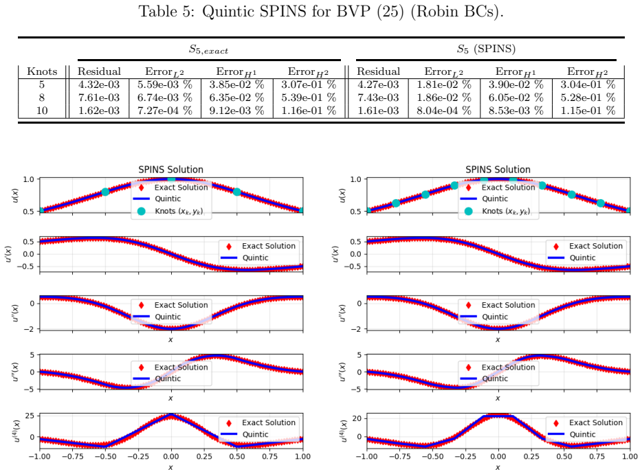
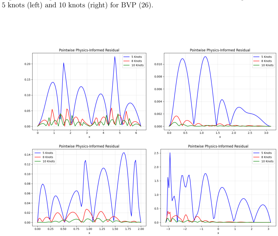
- [Numerical experiments] The numerical demonstrations do not report quantitative error norms, convergence rates with respect to the number of spline knots, or direct comparisons against standard finite-difference or collocation schemes. Without these data it is impossible to substantiate the repeated assertion of 'high accuracy' or to evaluate whether the observed residuals translate into small solution errors for the tested nonlinear problems.
minor comments (2)
- [Abstract] The abstract states that the method is demonstrated 'using cubic and quintic interpolating splines' but does not indicate the knot distributions or the precise number of degrees of freedom employed; adding this information would clarify the minimal-parameter claim.
- [Method] Notation for the spline basis functions and the residual loss functional is introduced without an explicit equation reference; a numbered display equation for the loss would improve readability.
Simulated Author's Rebuttal
We thank the referee for the constructive and detailed comments on our manuscript. We address each major comment below and indicate the specific revisions planned for the next version.
read point-by-point responses
-
Referee: The central claim that driving the physics-informed residual to near zero over the coefficients of a fixed cubic or quintic interpolating spline produces a high-accuracy solution presupposes that the unknown solution lies in (or is well approximated by) that low-dimensional spline space. No approximation-theoretic argument, error bound, or regularity assumption is supplied to justify this for arbitrary nonlinear second-order ODEs; the manuscript therefore provides no a-priori guarantee that the minimizer recovers an accurate approximation when the true solution exhibits layers, oscillations, or limited smoothness.
Authors: We acknowledge that the manuscript lacks an explicit approximation-theoretic justification or a priori error bounds. While cubic and quintic splines possess well-known approximation properties for sufficiently smooth functions, the nonlinear character of the ODEs complicates direct transfer of these results. In the revised manuscript we will add a short subsection in the methodology that recalls standard spline approximation results (O(h^4) for cubic splines on C^4 functions) and states the regularity assumptions under which the method is expected to converge. We will also include a brief discussion of limitations for solutions with limited smoothness or interior layers. revision: yes
-
Referee: The numerical demonstrations do not report quantitative error norms, convergence rates with respect to the number of spline knots, or direct comparisons against standard finite-difference or collocation schemes. Without these data it is impossible to substantiate the repeated assertion of 'high accuracy' or to evaluate whether the observed residuals translate into small solution errors for the tested nonlinear problems.
Authors: We agree that quantitative error measures and convergence data are necessary to support the accuracy claims. The present version relies primarily on visual comparisons and residual plots. In the revision we will augment the numerical experiments section with tables reporting L2 and L-infinity errors against exact solutions, convergence rates obtained by successively increasing the number of knots, and side-by-side comparisons with a standard second-order finite-difference scheme and a collocation method for the benchmark problems. revision: yes
Circularity Check
No significant circularity in SPINS derivation chain
full rationale
The paper defines SPINS as a direct numerical scheme that parameterizes the solution in a fixed spline basis (cubic or quintic interpolating), enforces boundary conditions by construction through the basis choice, and optimizes the spline coefficients by minimizing the physics-informed residual of the ODE. This chain is self-contained: the loss is derived from the differential equation itself rather than from data fits, and the reported accuracy on demonstrated examples follows from the optimization without reducing to a tautology or self-fit. No load-bearing self-citations, uniqueness theorems, or ansatz smuggling appear in the provided abstract or described method. The approach is a standard collocation-style method with spline basis and does not rename known results or import circular premises.
Axiom & Free-Parameter Ledger
Lean theorems connected to this paper
-
IndisputableMonolith/Cost/FunctionalEquation.leanwashburn_uniqueness_aczel unclear?
unclearRelation between the paper passage and the cited Recognition theorem.
SPINS approximates the solution u(x) using a spline S(x) of order q ... J(y) = 1/2 ∥F(·, S, S′, S″)∥₂ ... minimization problem whose objective function is J
-
IndisputableMonolith/Foundation/RealityFromDistinction.leanreality_from_one_distinction unclear?
unclearRelation between the paper passage and the cited Recognition theorem.
By replacing the neural network architecture of traditional PINNs with a structured spline basis
What do these tags mean?
- matches
- The paper's claim is directly supported by a theorem in the formal canon.
- supports
- The theorem supports part of the paper's argument, but the paper may add assumptions or extra steps.
- extends
- The paper goes beyond the formal theorem; the theorem is a base layer rather than the whole result.
- uses
- The paper appears to rely on the theorem as machinery.
- contradicts
- The paper's claim conflicts with a theorem or certificate in the canon.
- unclear
- Pith found a possible connection, but the passage is too broad, indirect, or ambiguous to say the theorem truly supports the claim.
Reference graph
Works this paper leans on
-
[1]
Nasri Cheaito and Ayman Mourad. An efficient forward-marching construction of the inter- polating splines.Computational Mathematics and Modeling, 2026. DOI: 10.1007/s10598- 026-09693-9
-
[2]
Differentiable spline approximations
Minsu Cho, Aditya Balu, Ameya Joshi, et al. Differentiable spline approximations. In Advances in Neural Information Processing Systems (NeurIPS), volume 34, pages 11122– 11135, 2021
work page 2021
-
[3]
Springer-Verlag, New York, 1978
Carl De Boor.A Practical Guide to Splines. Springer-Verlag, New York, 1978
work page 1978
-
[4]
Jim Douglas, Todd Dupont, and Lars Wahlbin. Optimall ∞ error estimates for galerkin approximations to solutions of two-point boundary value problems.Mathematics of Com- putation, 29(130):475–483, 1975
work page 1975
-
[5]
Antonella Falini, Giuseppe Alessio D’Inverno, Maria Lucia Sampoli, and Francesca Mazzia. Splines parameterization of planar domains by physics-informed neural networks.Mathe- matics, 11(10):2406, 2023
work page 2023
-
[6]
Charles A. Hall and Weston W. Meyer. Optimal error bounds for cubic spline interpolation. Journal of Approximation Theory, 16(2):105–122, 1976
work page 1976
-
[7]
Physics-informed machine learning.Nature Reviews Physics, 3(6):422–440, 2021
George E Karniadakis, Ioannis G Kevrekidis, Lu Lu, Paris Perdikaris, Sifan Wang, and Liu Yang. Physics-informed machine learning.Nature Reviews Physics, 3(6):422–440, 2021
work page 2021
-
[8]
Randall J LeVeque.Finite Difference Methods for Ordinary and Partial Differential Equa- tions: Steady-State and Time-Dependent Problems. SIAM, 2007
work page 2007
-
[9]
Maziar Raissi, Paris Perdikaris, and George E Karniadakis. Physics-informed neural net- works: A deep learning framework for solving forward and inverse problems involving non- linear partial differential equations.Journal of Computational Physics, 378:686–707, 2019
work page 2019
-
[10]
William E Schiesser.Spline Collocation Methods for Partial Differential Equations: With Applications in R. John Wiley & Sons, 2017
work page 2017
-
[11]
Martin H. Schultz.Spline Analysis. Prentice-Hall, Englewood Cliffs, NJ, 1973
work page 1973
-
[12]
Gilbert Strang and George J Fix.An Analysis of the Finite Element Method. Prentice-Hall, 1973. 25
work page 1973
-
[13]
Physics-informed spline learning for nonlinear dynamics discovery
Fangzheng Sun, Yang Liu, and Hao Sun. Physics-informed spline learning for nonlinear dynamics discovery. InProceedings of the Thirtieth International Joint Conference on Ar- tificial Intelligence (IJCAI-21), pages 2110–2117, 2021
work page 2021
-
[14]
Spline-pinn: Ap- proaching pdes without data using fast, physics-informed hermite-spline cnns
Nils Wandel, Michael Weinmann, Michael Neidlin, and Reinhard Klein. Spline-pinn: Ap- proaching pdes without data using fast, physics-informed hermite-spline cnns. InProceed- ings of the AAAI Conference on Artificial Intelligence, volume 36, pages 8529–8538, 2022
work page 2022
-
[15]
Zhuoyuan Wang, Raffaele Romagnoli, Jasmine Ratchford, and Yorie Nakahira. Physics- informed deep b-spline networks for dynamical systems.Transactions on Machine Learning Research, 2026. Accepted March 9, 2026. Available at arXiv:2503.16777
-
[16]
Olek C Zienkiewicz, Robert L Taylor, and Jianzhong Zhu.The Finite Element Method: Its Basis and Fundamentals. Elsevier, 7th edition, 2013. 26
work page 2013
discussion (0)
Sign in with ORCID, Apple, or X to comment. Anyone can read and Pith papers without signing in.