REVIEW 5 major objections 6 minor 1 cited by
Differences in the solar cycle variability of simple and complex active regions during 1996-2018
T0 review · 5 major / 6 minor · reviewed 2026-08-14 · deepseek-v4-flash
Pith's one-line read Complex active regions lag simple ones by about two years in each solar cycle, and their peak abundance is nearly identical across the two cycles.
desk verdict The two-year SAR/CAR lag is a real pattern in the daily SRS counts, but lifetime-weighted counting could produce it; the paper deserves revision and peer review. read the letter →
The pith
A machine-rendered reading of the paper's core claim, the machinery that carries it, and where it could break.
The reading
What carries the argument
The central object is the daily magnetic-complexity count: instead of assigning one complexity class to each active region at a single moment, the method adds one count of the region's current Mount Wilson class ($\alpha$, $\beta$, $\beta\gamma$, or $\beta\gamma\delta$) for every day the region appears on the disk. This lifetime-weighted daily counting is what separates the SAR and CAR time series and reveals the two-year lag, because a region that spends part of its life simple and part complex contributes to both groups. The comparison series is the monthly sunspot number, smoothed with a seven-month running average, and the load-bearing statistics are the peak timings, the correlation coefficients, and the cycle-to-cycle ratios of peak counts.
What would settle it
Compute monthly simple- and complex-region counts using a single complexity class per region, taken from the day of its maximum sunspot area; if the complex-region peak then coincides with the sunspot-number peak rather than lagging by two years, the lag is a product of the daily weighting. Splitting the record by observing era would further expose a classification-drift artifact if the two-year lag disappears in one sub-interval.
Extended reading notes
Core claim
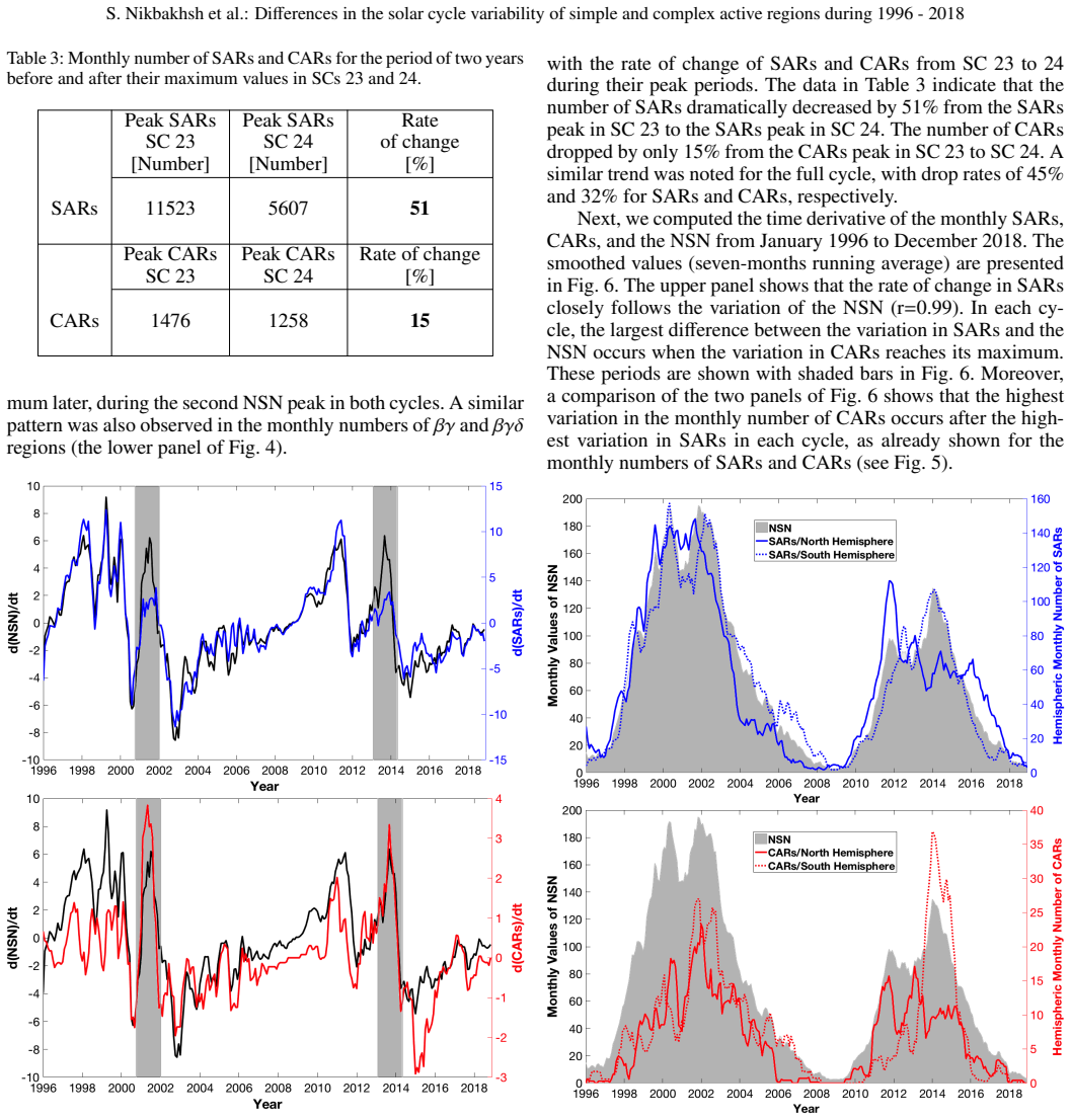
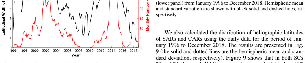
Using a newly developed daily counting method, in which each active region contributes one count per day and may change complexity class during its lifetime, the paper shows that monthly counts of simple active regions (SARs, classes $\alpha$ and $\beta$) track the reference sunspot number with correlation $r=0.99$ and peak in May 2000 during cycle 23 and December 2011 during cycle 24. Complex active regions (CARs, classes $\beta\gamma$ and $\beta\gamma\delta$) instead peak in November 2001 and January 2014, about two years later in each cycle, with a weaker correlation of $r=0.87$. From the two-year window around each peak, the CAR count drops only 15% between cycles 23 and 24, while the SAR count drops 51%; the same pattern holds over the full cycles, with drops of 32% and 45%. In both hemispheres the CAR peak occurs before the latitudinal width of the activity band starts to decrease, which the paper takes as evidence against the idea that complex regions appear because the activity band narrows. The paper concludes that the two dynamo processes compete during flux emergence: the cyclically varying large-scale dynamo dominates at solar maximum and produces mostly simple regions, while the cycle-independent small-scale dynamo becomes relatively more important in the declining phase and makes an increasing share of emerging flux complex.
Load-bearing premise
The analysis assumes that daily Mount Wilson complexity labels in the 22-year record are assigned consistently over time, and that counting each region once per day does not systematically shift complex regions to later in their lifetimes; if either fails, the two-year lag and the cycle-to-cycle stability of complex counts are artifacts.
Editorial extensions
If this is right
- Monthly counts of simple active regions become a near-perfect proxy for the sunspot cycle, so intervals where that correlation breaks down mark times when the complex-region contribution is changing.
- The two-year lag means each cycle's late maximum and early declining phase, not its peak, is when complex active regions are most abundant.
- The 15% versus 51% decline in peak counts implies that complex-region production is far more stable across cycles than bulk sunspot activity.
- Since complex regions are the more flare- and CME-productive class, the late-cycle CAR peak implies elevated eruptive activity roughly two years after sunspot maximum.
- The CAR peak occurring before the activity band narrows argues against the previously suggested mechanism that latitudinal compression creates complex regions.
Reading between the lines
- A natural test of the two-year lag is the next solar cycle: if the competition story is right, the complex-region peak of cycle 25 should again trail the sunspot-number peak by roughly two years.
- Recomputing the counts with one classification per region, taken from the day of maximum sunspot area, would isolate whether the daily lifetime-weighting method itself creates the lag; if the lag disappears, the dynamo interpretation would rest on a counting artifact.
- The near-constant complex-region peak suggests a complexity floor that is nearly independent of cycle strength; if real, the ratio of simple to complex peak counts is a more sensitive dynamo diagnostic than either count alone.
Signed reviews
Editorial analysis
A structured set of objections, weighed in public.
Referee Report
Summary. The paper analyzes NOAA/SRS daily active region (AR) data from January 1996 to December 2018, assigning each AR a Mount Wilson complexity class per day. It introduces a 'daily magnetic complexity approach' in which each region contributes one count for every day it appears in a given class, and then groups \u03b1 and \u03b2 classes as simple active regions (SARs) and \u03b2\u03b3 and \u03b2\u03b3\u03b4 as complex active regions (CARs). The main findings are: (i) monthly SAR numbers track the NOAA sunspot number (NSN) closely (r=0.99) and peak during the first NSN peak in each cycle (May 2000 in SC 23, December 2011 in SC 24); (ii) monthly CAR numbers peak about two years later, during the second NSN peak (November 2001 and January 2014); (iii) the total number of CARs in a four-year window around the CAR peak drops only 15% from SC 23 to SC 24, versus 51% for SARs (Table 3); (iv) CARs peak before the latitudinal width of the activity band starts to decrease (Fig. 8). The authors interpret these results as evidence for competition between a cyclic large-scale dynamo (LSD) and a cycle-independent small-scale dynamo (SSD), with the SSD gaining relative influence in the declining phase and producing the late, cycle-independent CAR peak. No model fitting is performed; all results are direct data reads.
Significance. If the reported peak lag and the near-cycle-independence of CAR counts hold, the paper would provide a new observational constraint on active region formation, suggesting that complex regions are a late-cycle phenomenon whose total rate is nearly independent of cycle strength. This would challenge the earlier Jaeggli & Norton (2016) interpretation that complex regions appear because the latitudinal activity band narrows, and it would support a surface small-scale dynamo contribution. The paper is laudably simple, uses a public dataset exclusively, fits no free parameters, and reports quantitative KS tests for the latitudinal distributions. Its central interpretation, however, rests on the unvalidated daily-count weighting: the two-year lag and the Table 3 cycle-to-cycle comparison are read from a lifetime-weighted series, and the 'peak before width decrease' claim in Fig. 8 is not statistically tested. These gaps do not invalidate the direct reading of the smoothed curves, but they materially weaken the causal interpretation.
major comments (5)
- [§2 and §3.2] The daily magnetic complexity approach counts each active region once for every day it is classified as α, β, βγ, or βγδ. As the paper acknowledges, this 'will emphasize long-lived ARs more than short-lived ones,' and §1 notes that an AR's complexity can change during its lifetime. The monthly CAR series is therefore not a measure of the emergence rate of complex regions but a lifetime-weighted sum of the days regions spend in complex classes. If complex classifications tend to be assigned late in a region's disk passage, or if the lifetime or classification duration of complex regions changes with cycle phase, the smoothed CAR curve can peak later than the underlying emergence and the cycle-to-cycle amplitude can be distorted. The central claims (the ~2-year SAR/CAR lag and the near-equal CAR peak counts in Table 3) are read directly from this series, with no per-AR control. A robustness check that counts each region once (e.g., at first appearance, at maximum area, or at maximum complexity) is necessary to support the LSD/SSD interpretation.
- [§2] The analysis treats the Mount Wilson classifications in the NOAA/SRS list as a stable, unbiased measure of magnetic complexity over 22 years. The paper does not discuss instrument or observer changes in the SOON network, nor does it test whether classification practice drifted over 1996-2018. A time-dependent classification threshold could produce an apparent phase lag or alter cycle-to-cycle amplitudes, directly affecting the main claims. Please provide at least a qualitative discussion of known data caveats, and preferably a consistency check against an independent classification source for a subset of the period.
- [§3.1 and Fig. 5] The Pearson correlations r=0.99 (SARs vs NSN) and r=0.87 (CARs vs NSN) are computed on seven-month moving averages without correcting for autocorrelation. With heavy smoothing, the effective number of independent samples is far below the number of monthly points, so the significance of these coefficients is overstated. In addition, r=0.99 for SARs is near-tautological because SARs comprise about 88% of all ARs and sunspot numbers are strongly driven by AR counts. The paper should report confidence intervals based on effective degrees of freedom, or correlations on unsmoothed or detrended data, and should avoid implying that 0.99 vs 0.87 is evidence of a different cycle relationship.
- [§3.4 and Fig. 8] The statement that CARs 'peaked before the latitudinal width starts to decrease' is an assessment of the figure with no quantitative test. There are no error bars, no peak-timing statistic, and no comparison against a null hypothesis (e.g., simultaneous peaking). Since this result is used to reject the Jaeggli & Norton (2016) hypothesis that complex regions increase because the latitude band narrows, it should be supported by a formal analysis, such as a cross-correlation of the two time series or a segmented regression on the width curve.
- [Table 3] The 'rate of change' from SC 23 to SC 24 is computed from four-year windows centered on the respective CAR and SAR peaks, but the windows are not symmetric in cycle phase and the two cycles have different shapes. The 15% drop in CAR counts versus 51% for SARs is presented without uncertainty. Given that monthly CAR peaks are around 50 (Fig. 5), a 15% difference may be within the noise, especially after smoothing. The paper should provide an estimate of the uncertainty on the peak-window sums (e.g., bootstrap on the unsmoothed monthly counts) before interpreting the near-equality as evidence for a cycle-independent SSD.
minor comments (6)
- [Abstract] The abstract contains small language errors: 'active region' should be 'active regions' in the Aims sentence, and 'decease' should be 'decrease' in the Results sentence.
- [§3.2 and Table 3] The phrase 'the period of two years before and after their maximum values' describes a four-year period; please clarify whether the maximum month is included in the window and whether the window is the same for both groups in each cycle.
- [Fig. 6] The shaded bars in Fig. 6 are described in the text as 'the periods when the largest difference between the time variation of SARs and the NSN happens,' but the caption does not explain how these periods are identified. Please specify the criterion used to draw the bars.
- [§3.1 and Fig. 5] The 'double peak' behavior is described qualitatively. It would be helpful to state how the two peaks are identified, for example whether they are local maxima in the smoothed curve with a minimum between them.
- [§2] The HELIO website is cited by URL in a footnote; please add a formal reference or access date for the dataset version used.
- [§3.3 and Fig. 7] The hemispheric curves in Fig. 7 may be difficult to distinguish in grayscale; using different line styles (solid vs dashed) or labels inside the panels would improve clarity.
Circularity Check
No significant circularity: the paper is an observational study with no fitted parameters, and its central comparisons are against external data.
full rationale
The paper's claims—SARs tracking the sunspot number, CARs peaking about two years later, and CAR peak abundance being cycle-to-cycle stable—are read directly from daily NOAA/SRS Mount Wilson classifications and compared with the independent Boulder/NOAA sunspot number. No parameter is fitted to the data and then renamed a prediction, no quantity is defined in terms of the quantity it is said to explain, and no load-bearing assertion rests on a self-citation. The r=0.99 SAR–NSN correlation is unsurprising because SARs dominate all ARs and both track global activity, but that is an observational near-equivalence, not a constructed reduction: the sunspot number is not built from the SRS complexity counts. The LSD/SSD discussion is explicitly presented as an interpretation ('We interpret this behavior in terms of the competition between...'), not as a derivation from the data, so it cannot be circular. The main limitations (unvalidated stability of SOON classifications over 22 years, lifetime weighting in the daily approach, and the absence of a quantitative test of the Fig. 8 timing claim) are data-quality and statistical-support issues, not circularity. Therefore the appropriate finding is no significant circularity.
Assumptions & free parameters
free parameters (2)
- Seven-month moving average smoothing window =
7 months, hand-chosen
- Four-year peak window (±2 years around each cycle maximum) =
2 years on each side, hand-chosen
assumptions (4)
- domain assumption The small-scale dynamo (SSD) generates a fluctuating magnetic field that is independent of the solar cycle.
- domain assumption The large-scale dynamo (LSD) dominates in the deeper convection zone and produces the cyclic large-scale field.
- domain assumption The Mount Wilson classifications in the NOAA/SRS list are a stable, unbiased measure of AR magnetic complexity over 1996-2018.
- domain assumption Lifetime-weighted daily counting does not bias the relative timing of the SAR and CAR peaks.
Cite this review
Pith. "Pith review of Differences in the solar cycle variability of simple and complex active regions during 1996-2018." pith.science (2026). https://pith.science/paper/PXIJ2VAN
@misc{pith2026190802226,
  author       = {Pith},
  title        = {Pith review of: Differences in the solar cycle variability of simple and complex active regions during 1996-2018},
  year         = {2026},
  howpublished = {\url{https://pith.science/paper/PXIJ2VAN}},
  note         = {Machine review of arXiv:1908.02226}
}
abstract
Aims. Our aim is to examine the solar cycle variability of magnetically simple and complex active region. Methods. We studied simple ($\alpha$ and $\beta$) and complex ($\beta\gamma$ and $\beta\gamma\delta$) active regions based on the Mount Wilson magnetic classification by applying our newly developed daily approach. We analyzed the daily number of the simple active regions (SARs) and compared that to the abundance of the complex active regions (CARs) over the entire solar cycle 23 and cycle 24 until December 2018. Results. We show that CARs evolve differently over the solar cycle from SARs. The time evolution of SARs and CARs on different hemispheres also shows differences, even though on average their latitudinal distributions are shown to be similar. The time evolution of SARs closely follows that of the sunspot number, and their maximum abundance was observed to occur during the early maximum phase, while that of the CARs was seen roughly two years later. We furthermore found that the peak of CARs was reached before the latitudinal width of the activity band starts to decease. Conclusions. Our results suggest that the active region formation process is a competition between the large-scale dynamo (LSD) and the small-scale dynamo (SSD) near the surface, the former varying cyclically and the latter being independent of the solar cycle. During solar maximum, LSD is dominant, giving a preference to SARs, while during the declining phase the relative role of SSD increases. Therefore, a preference for CARs is seen due to the influence of the SSD on the emerging flux.
Figures


Figures from the paper (4 more)


Forward citations
Cited by 1 Pith paper
-
Solar Cycle Variation of the Distribution of Photospheric Magnetic Flux Features
A smooth double power law, not a single power law, best fits the photospheric flux distribution over the full solar cycle; its large-scale slope varies with activity while the small-scale slope is stable.
Reference graph
Works this paper leans on
-
[1]
2013, Air Force Weather Agency Manual, http://static
Andrus, D. 2013, Air Force Weather Agency Manual, http://static. e-publishing.af.mil/production/1/afwa/publication/ afwaman15-1/afwaman15-1.pdf , page 37, Air Force Departmental Publishing Office
work page 2013
-
[2]
Balasubramaniam, K. S. & Henry, T. W. 2016, Sol. Phys., 291, 3123
work page 2016
-
[3]
Batchelor, G. K. 1950, Proceedings of the Royal Society of London Series A, 201, 405
work page 1950
-
[4]
Buehler, D., Lagg, A., & Solanki, S. K. 2013, A&A, 555, A33
2013
- [5]
-
[6]
2011, Journal of Geophysical Research (Space Physics), 116, A12108
Chen, C., Wang, Y ., Shen, C., et al. 2011, Journal of Geophysical Research (Space Physics), 116, A12108
2011
-
[7]
2016, Sol
Clette, F., Lefèvre, L., Cagnotti, M., Cortesi, S., & Bulling, A. 2016, Sol. Phys., 291, 2733
2016
-
[8]
Cortie, A. L. 1901, ApJ, 13, 260
1901
Show all 34 references
-
[9]
2014, MNRAS, 441, 2208
Guo, J., Lin, J., & Deng, Y . 2014, MNRAS, 441, 2208
2014
-
[10]
E., Ellerman, F., Nicholson, S
Hale, G. E., Ellerman, F., Nicholson, S. B., & Joy, A. H. 1919, ApJ, 49, 153
1919
-
[11]
Hale, G. E. & Nicholson, S. B. 1938, Magnetic observations of sunspots, 1917- 1924 ... (Washington, D.C. Carnegie institution of Washington, 1938.)
1938
-
[12]
Hathaway, D. H. 2015, Living Reviews in Solar Physics, 12, 4
2015
-
[13]
2014, Solar Origins of Space Weather and Space Climate (Springer)
Hernandez, G., Komm, R., Pevtsov, A., & Leibache, J. 2014, Solar Origins of Space Weather and Space Climate (Springer)
2014
-
[14]
Howard, R. F. 1989, Sol. Phys., 123, 271
1989
-
[15]
A., McAteer, R
Ireland, J., Young, C. A., McAteer, R. T. J., et al. 2008, Sol. Phys., 252, 121
2008
-
[16]
Jaeggli, S. A. & Norton, A. A. 2016, ApJ, 820, L11 Künzel, H. 1960, Astronomische Nachrichten, 285, 271
2016
-
[17]
McIntosh, P. S. 1990, Sol. Phys., 125, 251
1990
-
[18]
R., Delouille, V ., Li, J
Moon, K. R., Delouille, V ., Li, J. J., et al. 2016, Journal of Space Weather and Space Climate, 6, A3
2016
-
[19]
2013, Journal of Space Weather and Space Climate, 3, A21
Mursula, K., Manoharan, P., Nandy, D., Tanskanen, E., & Verronen, P. 2013, Journal of Space Weather and Space Climate, 3, A21
2013
-
[20]
1998, 140, 519
Neidig, D., Wiborg, P., Confer, M., et al. 1998, 140, 519
1998
-
[21]
Parker, E. N. 1955, ApJ, 122, 293
1955
-
[22]
& Szakaly, G
Petrovay, K. & Szakaly, G. 1993, A&A, 274, 543
1993
-
[23]
H., Teukolsky, S
Press, W. H., Teukolsky, S. A., Vetterling, W. T., & Flannery, B. P. 2007, Numer- ical Recipes: The Art of Scientific Computing (Cambridge University Press)
2007
-
[24]
2000, ApJ, 540, 583
Sammis, I., Tang, F., & Zirin, H. 2000, ApJ, 540, 583
2000
-
[25]
Smith, S. F. & Howard, R. 1968, 35, 33
1968
-
[26]
Spencer, J. B. 1965, Leaflet of the Astronomical Society of the Pacific, 9, 273
1965
-
[27]
C., Lee, T
Stenning, D. C., Lee, T. C. M., van Dyk, D. A., et al. 2013, Statistical Analysis and Data Mining: The ASA Data Science Journal, 6, 329
2013
-
[28]
& Dere, K
Subramanian, P. & Dere, K. P. 2001, ApJ, 561, 372
2001
-
[29]
& Kitai, R
Takizawa, K. & Kitai, R. 2015, Sol. Phys., 290, 2093
2015
-
[30]
1983, Sol
Tang, F. 1983, Sol. Phys., 89, 43
1983
-
[31]
Tang, F.,Howard, R., & Adkins, J. M. 1984, Sol. Phys., 91, 75 van Driel-Gesztelyi, L. & Green, L. M. 2015, Living Reviews in Solar Physics, 12, 1
1984
-
[32]
1938, ZAp, 16, 276
Waldmeier, M. 1938, ZAp, 16, 276
1938
-
[33]
& Liu, C
Wang, H. & Liu, C. 2015, Research in Astronomy and Astrophysics, 15, 145
2015
-
[34]
& Jingxiu, W
Zhongxian, S. & Jingxiu, W. 1994, Sol. Phys., 149, 105 Article number, page 9 of 9
1994
Reviewed August 14, 2026 · model on record in the stance chip above.
Discussion (0). Continue with ORCID to comment.