REVIEW 4 major objections 7 minor 1 cited by
Systematic Search for Long-Term Trends in Fermi-LAT Jetted Active Galactic Nuclei
T0 review · 4 major / 7 minor · reviewed 2026-08-10 · deepseek-v4-flash
Pith's one-line read A systematic search of Fermi-LAT light curves identifies 40 jetted active galactic nuclei with significant decade-long gamma-ray flux trends—32 linear and 8 quadratic—and finds that in about 80% of them the variability amplitude grows…
desk verdict A genuinely useful first systematic census of long-term gamma-ray trends in jetted AGN, but the 40-source count rests on R-squared measured on a smoothed trend and needs re-verification on raw fluxes. read the letter →
The pith
A machine-rendered reading of the paper's core claim, the machinery that carries it, and where it could break.
The reading
What carries the argument
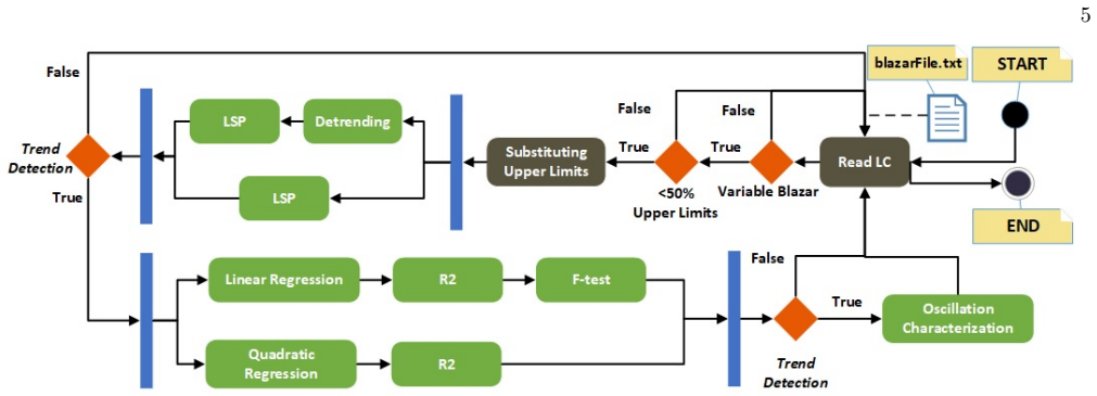
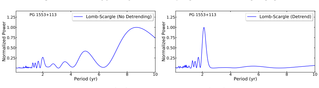
The detector is a two-stage pipeline. First, a Lomb-Scargle periodogram run on both the original and linearly detrended light curve preselects sources whose dominant frequency shifts by more than 20%, flagging possible trends. Then seasonal decomposition with a 40-bin period and multiplicative model extracts a smooth trend line; a linear or quadratic fit must reach R² ≥ 0.75, with an F-test (p ≤ 0.01) excluding a constant model. The pipeline also classifies oscillation behavior by regressing the flux of high-flux peaks against time, labeling oscillations additive when the slope is consistent with zero and multiplicative otherwise.
What would settle it
Take the 40 claimed trend sources and fit the same linear or quadratic models directly to the raw 28-day flux values, replacing upper limits by the paper's own likelihood-maximizing substitution or by a survival analysis, and recompute R² and the F-test p-value without any seasonal-decomposition smoothing; if a substantial fraction fail R² ≥ 0.75 on the raw data, the smoothed-trend criterion rather than an astrophysical trend would be doing the selection. A complementary check is to inject synthetic trends of known slope into real non-trending Fermi light curves and compare recovery rates when the fit is evaluated on raw versus smoothed data.
Extended reading notes
Core claim
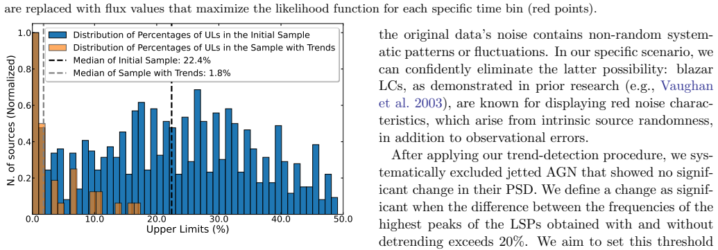
A systematic pipeline—Lomb-Scargle periodograms with and without detrending to flag frequency-domain changes, then seasonal decomposition to extract the smooth trend, then linear or quadratic fits with R² ≥ 0.75 and an F-test for nonzero slope—selects 40 of the 1,492 variable jetted AGN studied as showing long-term gamma-ray trends over roughly 10 years: 32 linear and 8 quadratic. Roughly 80% of these sources show multiplicative oscillations, where oscillation amplitude grows or shrinks with the trend, and the selected sources have very few upper limits (median 1.8%). The paper claims this is the first known sample of gamma-ray emitters with long-term trends of this nature and interprets the trends as possibly arising from supermassive-black-hole binary dynamics or from intrinsic jet phenomena such as magnetic reconnection or geometric Doppler-factor changes.
Load-bearing premise
The whole selection rests on the premise that the smooth trend extracted by the seasonal decomposition, and the R² computed from that smoothed line, faithfully represents the true astrophysical trend; the validation simulations use the same smoothing, so they never test whether a source that passes on the smoothed line would also pass on the raw 28-day light curve.
Editorial extensions
If this is right
- If correct, the 40 sources provide the first large sample for testing physical models of long-term gamma-ray trends, including supermassive-black-hole binary lump-driven accretion modulation and jet-internal mechanisms.
- Roughly 80% of trend sources show multiplicative oscillations; future periodicity searches in these objects must account for a trend-dependent oscillation amplitude or risk masking genuine quasi-periodic oscillations.
- The strong preference for linear (32) over quadratic (8) trends, and the low upper-limit fraction among selected sources, suggests trends are best seen in well-sampled light curves; real trends in sources with many upper limits may remain hidden.
- The flare-injection simulations show that bright, long-duration flares can destroy trend detection, implying the 40-source sample is a lower bound and additional trend sources may be found once flaring epochs are modeled or removed.
Reading between the lines
- The pipeline's reliance on a fixed 40-bin seasonality and an R² ≥ 0.75 threshold may select trends that are smooth by construction; an independent check using raw-data fits or Bayesian model comparison could reveal whether the true incidence of long-term trends is higher or lower than 40 in 1,492.
- The additive-versus-multiplicative classification, based on peak fluxes above 40–60% of maximum, could be extended to a full amplitude-trend correlation analysis using the entire light curve, which would test whether 'multiplicative' is a sharp dichotomy or a continuum.
- If multiplicative oscillations are common, the physical interpretation shifts: the same mechanism that drives the trend also modulates the variability amplitude, a pattern naturally predicted by geometric Doppler-factor changes but less naturally by a simple accretion-rate trend.
- A direct extension would apply the same pipeline to the next Fermi-LAT catalog release, and to optical and radio light curves of the same 40 objects, to test whether the gamma-ray trends persist and whether they are achromatic.
Signed reviews
Editorial analysis
A structured set of objections, weighed in public.
Referee Report
Summary. The manuscript reports a systematic search for long-term (~10 yr) linear and quadratic flux trends in the gamma-ray light curves of jetted AGN. From 3308 sources in 4FGL-DR2, a variability-index cut and an upper-limit-fraction cut select 1492 sources with 28-day binned light curves spanning 2008-2020. The detection pipeline compares Lomb-Scargle periodograms with and without linear detrending (requiring a >20% shift of the dominant peak), extracts a smooth trend with statsmodels seasonal_decompose (period=40, multiplicative), fits a line or parabola to that extracted trend and requires R^2 >= 75% with an F-test (p <= 0.01) on the slope, and classifies accompanying oscillations as additive or multiplicative. The result is a catalogue of 40 sources (32 linear, 8 quadratic, ~80% with multiplicative oscillations), an estimated 0.47% false-positive detection rate, and extensive injection-recovery tests under white, pink, red, and bending-power-law noise and under injected flares. Physical interpretations in terms of SMBH binaries and jet-intrinsic processes are discussed.
Significance. If the catalogue is correct, this is a valuable first census of long-lived monotonic gamma-ray trends in AGN and a useful target list for periodicity searches. The strengths are the scale and reproducibility of the processing (standard public packages throughout), the injection-recovery experiments of Sections 4.2-4.3, and the transparent internal diagnostics: Section 4.4 states that about 7 of the 1492 sources are expected to pass the pipeline spuriously, and Section 4.3 openly reports that flaring contamination suppresses trend recovery almost completely. Against this, the headline claim of 40 objects rests on an R^2 criterion computed on a smoothed surrogate of each light curve rather than on the observed fluxes (Section 3.3, Figures 5 and A1), and the paper's own FPDR implies that several of the 40 are likely spurious under the pipeline as built. Some of the flagged sources (e.g., PG 1553+113, 3C 84, BL Lac) are convincing from the displayed light curves, so the direction of the result is plausible, but the exact list and the count of 40 are not yet established.
major comments (4)
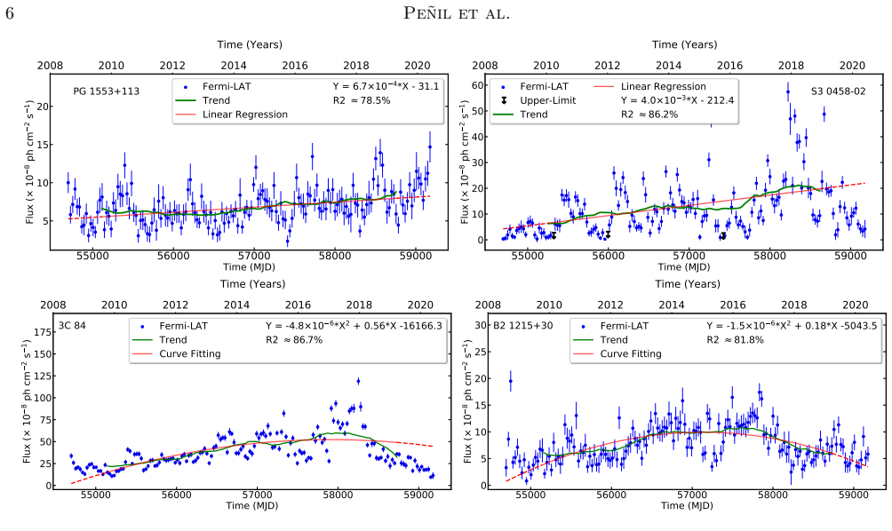
- [Section 3.3, Figures 5 and A1, Table 2] The R^2 selection is applied to the smoothed trend component returned by seasonal_decompose, not to the 28-day binned light curve. The Figure 5 caption states that the red line is 'the fit of the green line', where the green line is the trend extracted by seasonal_decompose (period=40, multiplicative); the R^2 values quoted in the panels and in Table 2 therefore quantify how well a line or parabola describes an already-smoothed, noise-reduced curve, not the fraction of observed flux variance explained by the trend. For a red-noise time series, a 40-bin moving-average trend can be smooth, extended, and monotonic-looking even when the raw flux has no sustained monotonic component, so the R^2>=75% filter can admit such sources and reject others whose raw scatter is large. The paper's own Table 3 is consistent with this reading: the R^2 stage passes 100% of simulated linear-trend light curves under every noise type, which would be implausible if R^2 were evaluated against the noisy simulated fluxes. The F-test on the slope (p<=0.01) is evaluated on the same smooth, autocorrelated residuals and does not carry its nominal significance. The 40-source list should be re-derived by fitting the linear/quadratic model directly to the 28-day fluxes, or at least complemented by a table of raw-data R^2 values for all 40 candidates.
- [Section 4.4] The paper's own FPDR, 0.47%, implies about 7 expected false positives among the 1492 sources, and no multiple-testing or false-discovery control is applied anywhere in the workflow. Since the pipeline reports 40 detections, about 17% of the list is expected to be spurious by the paper's calibration; the abstract's statement that the analysis 'identified 40 jetted AGN that exhibit long-term trends' is therefore stronger than the analysis supports. The authors should either report a corrected significance or an expected number of false positives per source (e.g., from the FPDR simulations) so that the reliability of the individual entries in Table 1 can be assessed.
- [Sections 4.2 and 4.4] The validation simulations inherit the smoothed-trend framework of Section 3.3, so they test internal consistency rather than the premise that the extracted trend represents the true astrophysical signal. Additionally, the slope ranges used to generate the simulated light curves in Section 4.2 are drawn from the detected values in Table 2, making the quoted recovery efficiencies conditional on the parameter ranges the search is meant to establish. Neither point is circular in the definition of the target (no result is defined through a fitted parameter), but both limit the evidential weight of the 'total detection' rates; re-running the recovery and FPDR simulations with the raw-data R^2 criterion would directly test the load-bearing assumption.
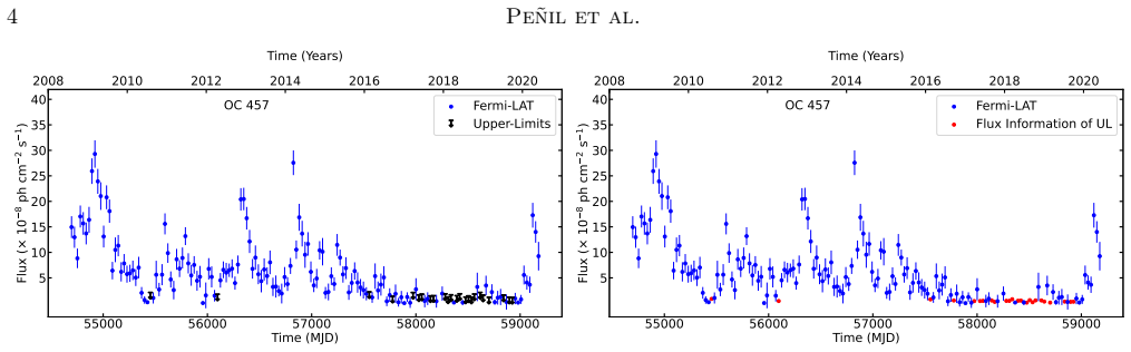
- [Section 3.1 and Figure 1] Upper-limit bins are replaced with the flux that maximizes the likelihood for that bin, a censoring treatment whose effect on fitted slopes is not modeled in the simulations of Sections 4.2-4.4. If such bins cluster in one part of the light curve, the substituted values can bias the estimated trend slope; the trend sample's low upper-limit fraction (median 1.8%, Figure 2) mitigates this risk but does not eliminate it. A robustness check recomputing the fits with upper limits either removed or replaced by the 95% upper-limit values would establish that the slopes and the membership of the 40-source list do not depend on this choice.
minor comments (7)
- [Section 4.2 and 4.1] Section 4.2 contains the typo 'liner-trend detection' (should be 'linear-trend'), and Section 4.1 refers to 'Table 110' where Table 1 is meant; the table captions in the text also render as 'T able 1' and 'T able 2' with an erroneous space.
- [Table 2] The printed uncertainties for AP Librae ('pm 4x10⁵') and B2 1520+31 ('pm 2x10⁴') appear to be missing the minus sign on the exponent (presumably 10^-5 and 10^-4); the same formatting issue affects several other entries where exponents are rendered without signs.
- [Figure A1] The last panel is labeled 'PKS 2345 16' with a missing minus sign, and several panels show y-axis tick labels like '5 0 5 10' that suggest negative flux values without explanation in the text.
- [Section 3.3] The sentence giving units has a parenthesis error ('are 10^-8 ph cm^-2 s^-1 days^-2), for...') and does not state the 10^-8 factor for the units of c, which would be helpful for readers using Table 2.
- [Section 4.1] The text reads 'Therefore, The remaining 8 sources' with an incorrect capital letter, and the paragraph beginning 'Analyzing the oscillatory behavior within this sample' is a sentence fragment.
- [Abstract and Section 3.3] The abstract says the trends span approximately 10 years while the data span 12 years; because seasonal_decompose drops roughly 40 bins at the edges (noted in the Figure 5 caption), the epoch over which the trend is actually constrained should be stated explicitly.
- [Section 3.3] The choice period=40 in seasonal_decompose (about 3.1 years) determines which timescales are assigned to the 'seasonal' component and which remain in the 'trend'; a brief justification of this choice or a robustness test with another period would strengthen the methodology.
Circularity Check
Mild self-referential validation in Section 4.2; central 40-source search is independent and not circular.
-
other
[Section 4.2, Evaluation of methods against noise]
"For linear trends, we randomly select slope values from the range of 1x10^{-3} to 9x10^{-3}, as most of the detected linear trends fall within this range (Table 2)."
The noise-recovery simulations calibrate the 'true' injected linear trends using slope values taken from the 40 detected sources in Table 2, and the same pipeline is then applied to measure recovery efficiency. The reported total detection rates therefore measure how often the pipeline re-finds trends drawn from its own detection sample, rather than independently validating that the detected trends are real. This is a minor validation circularity: it does not force the 40-source list itself, since the real-LC selections are made before and independently of these simulations, but it makes the Section 4.2 efficiency numbers partly self-referential.
full rationale
The paper's central claim is an empirical search over Fermi-LAT light curves: the 40-source list is produced by applying a fixed pipeline (variability index, upper-limit fraction, Lomb-Scargle change, seasonal-decompose trend extraction, R2 >= 75% on the extracted trend, and F-test) to real data, and the pipeline could in principle return zero sources. No target quantity is defined in terms of a fitted parameter, and no prediction is statistically forced by a fit. The R2 >= 75% criterion is applied to the seasonal_decompose trend component rather than to the raw 28-day fluxes; this is a statistical-validity concern about how well the smoothed surrogate represents the data, not a circular reduction, because the decomposition is not derived from the linear/quadratic model being tested. The false-positive rate (0.47%) is estimated from simulated LCs built from 100 non-trend blazars with their own PSDs, which is an independent check of the selection stage. The only mild circularity is in the noise-injection validation of Section 4.2, where the injected linear slopes are drawn from the range of detected slopes in Table 2; this makes the reported recovery efficiencies partly self-referential, although it does not affect the 40-source detection itself. Self-citations to Penil et al. (2020, 2022, 2024) are used for methodology, period uncertainties, and background context, and are not load-bearing for the main claim. Score 1.
Assumptions & free parameters
free parameters (6)
- R-squared selection threshold =
0.75
- LSP peak frequency shift threshold =
20%
- seasonal_decompose period =
40 bins (~3.1 years)
- F-test p-value for linear slope =
0.01
- F-test p-value for oscillation classification =
0.05
- find_peaks thresholds =
40%-60% of max flux, at least 3 peaks
assumptions (5)
- domain assumption The 4FGL-DR2 variability index threshold of 18.48 correctly identifies intrinsically variable jetted AGN
- ad hoc to paper The seasonal_decompose multiplicative trend line represents the true astrophysical long-term trend
- domain assumption Replacing upper limits with the likelihood-maximizing flux value does not bias trend estimation
- domain assumption Simulated light curves generated with the Emmanoulopoulos et al. (2013) method and power-law PSDs reproduce real blazar red noise
- standard math Linear detrending before Lomb-Scargle is sufficient to avoid trend-induced false periodicity
Cite this review
Pith. "Pith review of Systematic Search for Long-Term Trends in Fermi-LAT Jetted Active Galactic Nuclei." pith.science (2026). https://pith.science/paper/Q22GBN2T
@misc{pith2026250101310,
  author       = {Pith},
  title        = {Pith review of: Systematic Search for Long-Term Trends in Fermi-LAT Jetted Active Galactic Nuclei},
  year         = {2026},
  howpublished = {\url{https://pith.science/paper/Q22GBN2T}},
  note         = {Machine review of arXiv:2501.01310}
}
abstract
Jetted Active Galactic Nuclei (AGN) exhibit variability across a wide range of time scales. Traditionally, this variability can often be modeled well as a stochastic process. However, in certain cases, jetted AGN variability displays regular patterns, enabling us to conduct investigations aimed at understanding its origins. Additionally, a novel type of variability has emerged in jetted AGN lightcurves, specifically, the observation of a long-term trend characterized by a linear increase of the flux with time in blazars such as PG 1553+113, which is among the objects most likely to display periodic behavior. In this paper, we present the results of a systematic search for long-term trends, spanning $\approx$10\, years, utilizing 12 years of Fermi-LAT observations. The study is focused on detecting the presence of linear or quadratic long-term trends in a sample of 3308 jetted AGN. Our analysis has identified 40 jetted AGN that exhibit long-term trends, each with distinct properties, which we also characterize in this study. These long-term trends may originate from the dynamics of a supermassive black hole binary system, or they could be the result of intrinsic phenomena within the jet itself. Our findings can help in addressing questions pertaining to the astrophysical origins of variability and periodicity within jetted AGN.
Figures
Figures from the paper (2 more)
Forward citations
Cited by 1 Pith paper
-
Profile Analysis of the Multiwavelength 2.1-year Oscillations of PG 1553+113
The ~2.1-year oscillations of blazar PG 1553+113 are broad, structured envelopes with non-repeating substructure, not a single self-similar wave.
Reference graph
Works this paper leans on
-
[1]
A., Ackermann, M., Ajello, M., et al
Abdo, A. A., Ackermann, M., Ajello, M., et al. 2010, ApJ, 722, 520, doi: 10.1088/0004-637X/722/1/520 Abdollahi, S., Ackermann, M., Ajello, M., et al. 2017, ApJ, 846, 34, doi: 10.3847/1538-4357/aa8092 Abdollahi, S., Acero, F., Ackermann, M., et al. 2020, ApJS, 247, 33, doi: 10.3847/1538-4365/ab6bcb Ackermann, M., Ajello, M., Albert, A., et al. 2015, ApJL, ...
-
[3]
a” (10 −8 ph cm−2 s−1 days−2), “b
Each AGN is characterized by the type of trend (linear or Quadratic) and type of oscillations (additive or multiplicative). “a” (10 −8 ph cm−2 s−1 days−2), “b” (10 −8 ph cm−2 s−1 days−1), and “c” (10 −8 ph cm−2 s−1) are the fitting parameters. Finally, the R 2 criterion is included. Association Name Trend Topology a b c R2 PKS 0047+023 Linear Additive – 8...
work page 1936
-
[4]
Fermi-LAT Upper-Limit Trend Linear Regression Y = 8.8×10 4*X - 46.5 R2 85.4% 2008 2010 2012 2014 2016 2018 2020 Time (Years) PKS 0047+023 55000 56000 57000 58000 59000 Time (MJD) 0 5 10 15 20 25 30Flux (× 10 8 ph cm 2 s
work page 2008
-
[5]
Fermi-LAT Upper-Limit Trend Linear Regression Y = -1.9×10 3*X + 116.3 R2 75.9% 2008 2010 2012 2014 2016 2018 2020 Time (Years) OC 457 55000 56000 57000 58000 59000 Time (MJD) 0 5 10 15Flux (× 10 8 ph cm 2 s
work page 2008
-
[6]
Fermi-LAT Upper-Limit Trend Linear Regression Y = 1.1×10 3*X - 61.4 R2 83.5% 2008 2010 2012 2014 2016 2018 2020 Time (Years) ZS 0214+083 55000 56000 57000 58000 59000 Time (MJD) 0 5 10 15 20 25Flux (× 10 8 ph cm 2 s
work page 2008
-
[7]
Fermi-LAT Trend Curve Fitting Y = 9.9×10 7*X2 + -0.11*X +3219.9 R2 81.6% 2008 2010 2012 2014 2016 2018 2020 Time (Years) PKS 0215+015 55000 56000 57000 58000 59000 Time (MJD) 0 10 20 30 40Flux (× 10 8 ph cm 2 s
work page 2008
-
[8]
Fermi-LAT Upper-Limit Trend Linear Regression Y = -2.0×10 3*X + 122.4 R2 76.6% 2008 2010 2012 2014 2016 2018 2020 Time (Years) 3C 66A 55000 56000 57000 58000 59000 Time (MJD) 0 5 10 15 20 25 30 35Flux (× 10 8 ph cm 2 s
work page 2008
-
[9]
Fermi-LAT Upper-Limit Trend Linear Regression Y = -3.2×10 3*X + 188.6 R2 86.4% 2008 2010 2012 2014 2016 2018 2020 Time (Years) PKS 0244-47 55000 56000 57000 58000 59000 Time (MJD) 0 10 20 30 40 50Flux (× 10 8 ph cm 2 s
work page 2008
Show all 39 references
-
[10]
Fermi-LAT Upper-Limit Trend Linear Regression Y = -3.2×10 3*X + 191.3 R2 83.2% 2008 2010 2012 2014 2016 2018 2020 Time (Years) PKS 0250-22 55000 56000 57000 58000 59000 Time (MJD) 0 5 10 15 20 25 30 35Flux (× 10 8 ph cm 2 s
2008
-
[11]
Light curves of the jetted AGN presented in Table
Fermi-LAT Upper-Limit Trend Linear Regression Y = 1.0×10 3*X - 52.4 R2 80.4% 2008 2010 2012 2014 2016 2018 2020 Time (Years) PKS 0405-385 Figure A1. Light curves of the jetted AGN presented in Table
2008
-
[12]
Fermi-LAT Upper-Limit Trend Linear Regression Y = -2.5×10 3*X + 149.0 R2 77.3% 2008 2010 2012 2014 2016 2018 2020 Time (Years) PKS 0420-01 55000 56000 57000 58000 59000 Time (MJD) 5 0 5 10 15 20 25 30 35Flux (× 10 8 ph cm 2 s
2008
-
[13]
Fermi-LAT Upper-Limit Trend Linear Regression Y = -1.8×10 3*X + 111.6 R2 79.1% 2008 2010 2012 2014 2016 2018 2020 Time (Years) PKS 0446+11 55000 56000 57000 58000 59000 Time (MJD) 0 5 10 15 20 25 30 35Flux (× 10 8 ph cm 2 s
2008
-
[14]
Fermi-LAT Trend Linear Regression Y = 2.0×10 3*X - 107.6 R2 84.9% 2010 2012 2014 2016 2018 2020 Time (Years) PKS 0447-439 55000 56000 57000 58000 59000 Time (MJD) 0 5 10 15 20 25 30Flux (× 10 8 ph cm 2 s
2010
-
[15]
Fermi-LAT Upper-Limit Linear Regression Trend Y = -1.8×10 3*X + 106.8 R2 86.9% 2008 2010 2012 2014 2016 2018 Time (Years) PKS 0601-70 55000 56000 57000 58000 59000 Time (MJD) 0.0 2.5 5.0 7.5 10.0 12.5 15.0 17.5Flux (× 10 8 ph cm 2 s
2008
-
[16]
Fermi-LAT Trend Linear Regression Y = 6.9×10 4*X - 36.5 R2 91.6% 2008 2010 2012 2014 2016 2018 2020 Time (Years) 1ES 0647+250 55000 56000 57000 58000 59000 Time (MJD) 0 10 20 30 40Flux (× 10 8 ph cm 2 s
2008
-
[17]
Fermi-LAT Upper-Limit Trend Linear Regression Y = -1.8×10 3*X + 105.5 R2 79.5% 2008 2010 2012 2014 2016 2018 2020 Time (Years) B2 0716+33 55000 56000 57000 58000 59000 Time (MJD) 0 10 20 30 40 50 60Flux (× 10 8 ph cm 2 s
2008
-
[18]
Fermi-LAT Upper-Limit Trend Linear Regression Y = -1.9×10 3*X + 115.6 R2 78.4% 2008 2010 2012 2014 2016 2018 2020 Time (Years) PKS 0805-07 55000 56000 57000 58000 59000 Time (MJD) 0 5 10 15 20 25Flux (× 10 8 ph cm 2 s
2008
-
[19]
(Continued)
Fermi-LAT Trend Linear Regression Y = 7.9×10 4*X - 39.5 R2 76.5% 2008 2010 2012 2014 2016 2018 2020 Time (Years) OJ 014 Figure A1. (Continued). 20 Pe˜nil et al. 55000 56000 57000 58000 59000 Time (MJD) 0 10 20 30 40 50 60 70 80Flux (× 10 8 ph cm 2 s
2008
-
[20]
Fermi-LAT Upper-Limit Trend Linear Regression Y = -3.3×10 3*X + 198.1 R2 82.6% 2008 2010 2012 2014 2016 2018 2020 Time (Years) PMN J0948+0022 55000 56000 57000 58000 59000 Time (MJD) 0 10 20 30 40 50Flux (× 10 8 ph cm 2 s
2008
-
[21]
Fermi-LAT Upper-Limit Trend Linear Regression Y = -2.3×10 3*X + 139.9 R2 80.4% 2008 2010 2012 2014 2016 2018 2020 Time (Years) 4C +01.28 55000 56000 57000 58000 59000 Time (MJD) 0 5 10 15 20 25 30Flux (× 10 8 ph cm 2 s
2008
-
[22]
Fermi-LAT Trend Curve Fitting Y = 1.7×10 6*X2 + -0.19*X +5464.5 R2 85.7% 2008 2010 2012 2014 2016 2018 2020 Time (Years) PKS 1101-536 55000 56000 57000 58000 59000 Time (MJD) 0 50 100 150 200 250 300 350Flux (× 10 8 ph cm 2 s
2008
-
[23]
Fermi-LAT Upper-Limit Trend Linear Regression Y = -2.1×10 2*X + 1208.7 R2 84.0% 2008 2010 2012 2014 2016 2018 2020 Time (Years) 4C +21.35 55000 56000 57000 58000 59000 Time (MJD) 0 10 20 30 40Flux (× 10 8 ph cm 2 s
2008
-
[24]
Fermi-LAT Upper-Limit Trend Linear Regression Y = 1.4×10 3*X - 75.7 R2 84.2% 2008 2010 2012 2014 2016 2018 2020 Time (Years) NVSS J141922-083830 55000 56000 57000 58000 59000 Time (MJD) 5 10 15 20 25Flux (× 10 8 ph cm 2 s
2008
-
[25]
Fermi-LAT Trend Linear Regression Y = -1.1×10 3*X + 69.8 R2 82.3% 2008 2010 2012 2014 2016 2018 2020 Time (Years) PKS 1424+240 55000 56000 57000 58000 59000 Time (MJD) 0 5 10 15 20 25Flux (× 10 8 ph cm 2 s
2008
-
[26]
Fermi-LAT Upper-Limit Linear Regression Trend Y = 1.2×10 3*X - 64.5 R2 81.7% 2008 2010 2012 2014 2016 2018 2020 Time (Years) TXS 1452+516 55000 56000 57000 58000 59000 Time (MJD) 10 20 30 40 50Flux (× 10 8 ph cm 2 s
2008
-
[27]
(Continued)
Fermi-LAT Trend Linear Regression Y = 1.1×10 3*X - 55.7 R2 82.3% 2008 2010 2012 2014 2016 2018 2020 Time (Years) AP Librae Figure A1. (Continued). 21 55000 56000 57000 58000 59000 Time (MJD) 0 20 40 60 80 100Flux (× 10 8 ph cm 2 s
2008
-
[28]
Fermi-LAT Trend Linear Regression Y = -1.1×10 2*X + 670.6 R2 94.3% 2008 2010 2012 2014 2016 2018 2020 Time (Years) B2 1520+31 55000 56000 57000 58000 59000 Time (MJD) 0 5 10 15 20Flux (× 10 8 ph cm 2 s
2008
-
[29]
Fermi-LAT Upper-Limit Linear Regression Trend Y = 1.1×10 3*X - 57.2 R2 79.1% 2010 2012 2014 2016 2018 2020 Time (Years) GB6 J1542+6129 55000 56000 57000 58000 59000 Time (MJD) 0.0 2.5 5.0 7.5 10.0 12.5 15.0 17.5Flux (× 10 8 ph cm 2 s
2010
-
[30]
Fermi-LAT Trend Curve Fitting Y = 5.6×10 7*X2 + -0.06*X +1840.8 R2 88.4% 2008 2010 2012 2014 2016 2018 2020 Time (Years) SBS 1646+499 55000 56000 57000 58000 59000 Time (MJD) 0 20 40 60 80 100Flux (× 10 8 ph cm 2 s
2008
-
[31]
Fermi-LAT Upper-Limit Trend Linear Regression Y = -1.9×10 3*X + 121.7 R2 75.3% 2008 2010 2012 2014 2016 2018 2020 Time (Years) PKS 1730-13 55000 56000 57000 58000 59000 Time (MJD) 0 10 20 30 40Flux (× 10 8 ph cm 2 s
2008
-
[32]
Fermi-LAT Upper-Limit Trend Linear Regression Y = 3.2×10 3*X - 172.3 R2 78.2% 2008 2010 2012 2014 2016 2018 2020 Time (Years) PKS 1936-623 55000 56000 57000 58000 59000 Time (MJD) 0 5 10 15 20 25Flux (× 10 8 ph cm 2 s
2008
-
[33]
Fermi-LAT Upper-Limit Trend Linear Regression Y = 1.6×10 3*X - 83.7 R2 81.7% 2008 2010 2012 2014 2016 2018 2020 Time (Years) MH 2136-428 55000 56000 57000 58000 59000 Time (MJD) 0 25 50 75 100 125 150 175Flux (× 10 8 ph cm 2 s
2008
-
[34]
Fermi-LAT Trend Linear Regression Y = 5.8×10 3*X - 295.8 R2 88.6% 2008 2010 2012 2014 2016 2018 2020 Time (Years) BL Lac 55000 56000 57000 58000 59000 Time (MJD) 0 10 20 30 40Flux (× 10 8 ph cm 2 s
2008
-
[35]
(Continued)
Fermi-LAT Upper-Limit Trend Linear Regression Y = 9.3×10 4*X - 49.0 R2 76.9% 2008 2010 2012 2014 2016 2018 2020 Time (Years) PKS B2258-022 Figure A1. (Continued). 22 Pe˜nil et al. 55000 56000 57000 58000 59000 Time (MJD) 0 10 20 30 40 50Flux (× 10 8 ph cm 2 s
2008
-
[36]
Fermi-LAT Upper-Limit Trend Linear Regression Y = -3.0×10 3*X + 180.4 R2 84.2% 2008 2010 2012 2014 2016 2018 2020 Time (Years) B2 2308+34 55000 56000 57000 58000 59000 Time (MJD) 0 10 20 30 40 50 60Flux (× 10 8 ph cm 2 s
2008
-
[37]
Fermi-LAT Trend Curve Fitting Y = -1.8×10 6*X2 + 0.21*X -5854.2 R2 75.3% 2008 2010 2012 2014 2016 2018 2020 Time (Years) PKS 2320-035 55000 56000 57000 58000 59000 Time (MJD) 5 0 5 10 15 20 25 30Flux (× 10 8 ph cm 2 s
2008
-
[38]
Fermi-LAT Trend Curve Fitting Y = 8.5×10 7*X2 + -0.1*X +2754.6 R2 87.7% 2008 2010 2012 2014 2016 2018 2020 Time (Years) PMN J2331-2148 55000 56000 57000 58000 59000 Time (MJD) 0 20 40 60 80Flux (× 10 8 ph cm 2 s
2008
-
[39]
(Continued)
Fermi-LAT Trend Curve Fitting Y = 1.9×10 6*X2 + -0.22*X +6128.2 R2 87.1% 2008 2010 2012 2014 2016 2018 2020 Time (Years) PKS 2345 16 Figure A1. (Continued)
2008
-
[391]
2011, Journal of Astrophysics and Astronomy, 32, 139, doi: 10.1007/s12036-011-9072-x Valverde, J., Horan, D., Bernard, D., et al
https://arxiv.org/abs/astro-ph/9609023 Urry, M. 2011, Journal of Astrophysics and Astronomy, 32, 139, doi: 10.1007/s12036-011-9072-x Valverde, J., Horan, D., Bernard, D., et al. 2020, ApJ, 891, 170, doi: 10.3847/1538-4357/ab765d Vaughan, S., Edelson, R., Warwick, R. S., & Uttl...
2011 arXiv
Reviewed August 10, 2026 · model on record in the stance chip above.
Discussion (0). Continue with ORCID to comment.