REVIEW 3 major objections 5 minor 42 references
Probabilistic Forecasting of the Arctic Sea Ice Edge with Contour Modeling
T0 review · 3 major / 5 minor · reviewed 2026-08-14 · deepseek-v4-flash
Pith's one-line read The paper's central claim is that Mixture Contour Forecasting post-processes dynamical ensemble output into calibrated probabilistic sea ice forecasts by modeling the ice edge itself as a contour, blended with recent climatology.
desk verdict A genuinely new contour-based post-processing method for Arctic sea ice forecasting that meets its main claim, but the comparison to TAQM lacks statistical support. read the letter →
The pith
A machine-rendered reading of the paper's core claim, the machinery that carries it, and where it could break.
The reading
What carries the argument
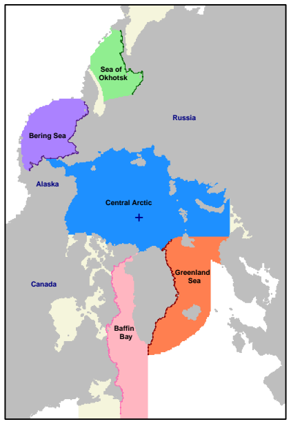
The central object is the contour representation: a sea ice edge is encoded by distances from land-based boundary points along a fixed set of parallel lines (or, in the Central Arctic, radial lines from a central point), converted to logit-scale ice-covered proportions. A Bayesian hierarchical model with an exponential covariance puts a prior on the mean contour informed by the Contour-Shifted ensemble forecast, and an EM-fitted mixture weight blends the resulting contour distribution with recent climatology. This representation concentrates modeling effort on the boundary, where forecast error is concentrated, and makes the forecast intrinsically probabilistic.
What would settle it
A direct stress test: refit MCF on the ten years before a known step change in Arctic sea ice variability, such as a season with an extreme minimum following rapid thinning, and compare reliability curves against those before the step; if observed frequencies of ice at forecast probabilities near 0.5 deviate from the diagonal, the stationary-window and linear-trend assumptions are the cause.
Extended reading notes
Core claim
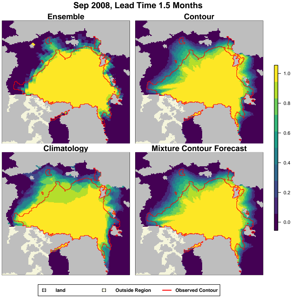
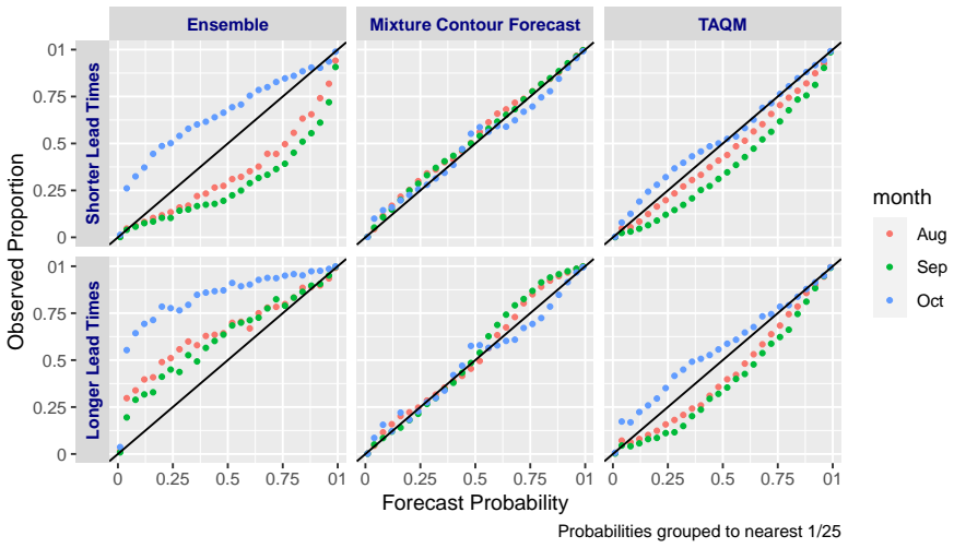
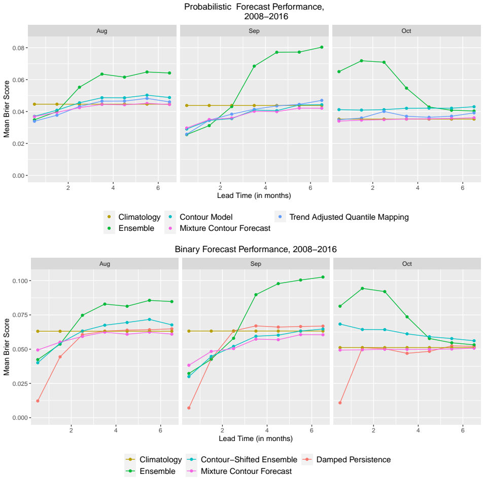
The paper claims that a forecast distribution for the sea ice edge can be built by treating the edge as an ordered set of points on fixed lines and modeling, for each line, the logit-transformed proportion of the line that is ice-covered as multivariate normal with an exponential covariance. The mean is anchored by a Contour-Shifted ensemble forecast, and the posterior over contours is mixed with a ten-year climatology in a finite mixture whose weight is estimated by maximum likelihood. Evaluated on SEAS5 dynamical ensemble output for 2008-2016 at lead times of 0.5 to 6.5 months, MCF's reliability diagrams sit closer to the diagonal than the raw ensemble's, and its area-weighted Brier scores are generally as good as or better than reference forecasts, with the largest gains at short lead times and in the peak-shipping months around September.
Load-bearing premise
The forecast distribution for a future year is built on the assumption that the contour distribution is stationary over the preceding ten years and that the trend in the difference between ensemble and observed contours is linear, so any nonlinear change in variability or bias will miscenter the prior and degrade calibration.
Editorial extensions
If this is right
- At lead times of 0.5 to 1.5 months, MCF's reliability curves are closer to the diagonal than the raw ensemble's, so mariners can treat its forecast probabilities as calibrated odds of encountering ice.
- In peak-shipping months MCF improves Brier scores over the raw ensemble and the contour-only model, and its accuracy reaches or exceeds climatology at longer leads as the mixture shifts weight away from the ensemble.
- The mixture weight automatically shifts toward the contour model at short lead times and near the September minimum, and toward climatology when the ensemble is weak, giving a principled way to blend model and observations.
- For binary 'is ice present' decisions, MCF matches or beats the Contour-Shifted ensemble and is substantially better in cases where the ensemble forecast is poor.
Reading between the lines
- Because the contour representation concentrates uncertainty on the boundary, the same modeling strategy could be applied to other geophysical edges where forecast error concentrates, such as the Antarctic sea ice edge or seasonal snow lines; the paper does not test these settings.
- The ten-year stationarity and linear-trend assumptions imply a testable vulnerability: in a decade with accelerating ice loss, the prior mean will lag, so an adaptive training-window length or an ensemble-informed covariance term may be needed.
- With calibrated probabilities, a natural next step is route optimization that minimizes expected cost under asymmetric penalties for hitting ice versus detouring; the paper mentions this possibility but does not implement it.
- The method's transfer to other ensembles is plausible since it uses no ensemble-specific features, but its performance gain over the raw ensemble could shrink or grow depending on the ensemble's initial calibration; that is an empirical question the paper leaves open.
Signed reviews
Editorial analysis
A structured set of objections, weighed in public.
Referee Report
Summary. The paper introduces Mixture Contour Forecasting (MCF), a post-processing method for probabilistic sea ice forecasts. The method first builds a Bayesian model of the sea ice edge contour, with a prior informed by a bias-corrected dynamic ensemble forecast (Contour Shifting), and then combines the contour distribution with a recent-climatology distribution via a weight estimated by maximum likelihood. The authors evaluate MCF on ECMWF SEAS5 forecasts for 2008-2016 at lead times from 0.5 to 6.5 months, comparing against the raw ensemble, climatology, the contour model alone, Trend Adjusted Quantile Mapping (TAQM), and a damped persistence forecast. The evaluation uses a rolling temporal holdout, reliability diagrams, and area-weighted Brier scores. The paper claims that at short lead times MCF is better calibrated than the unadjusted ensemble and other statistical reference forecasts, and that it is also competitive or better in accuracy, particularly in peak shipping months.
Significance. If the claims hold, MCF is a practically useful method for operational Arctic sea ice forecasting, addressing a real need for calibrated probabilistic forecasts of the ice edge. The paper's strengths include a genuine out-of-sample evaluation with temporally rolling training windows, use of multiple reference methods, and publicly available code. The contour-based representation is a reasonable modeling choice for the sea ice edge, and the mixture with climatology is a sensible way to blend dynamical and statistical information. However, the statistical evidence supporting the headline comparative claims is incomplete: the reported score differences lack uncertainty quantification and most modeling choices are not subjected to sensitivity analysis.
major comments (3)
- [§4.5, Eq. (30); Figs. 6-7] The central comparative claim that MCF is 'better calibrated and more accurate' than references rests entirely on point estimates. The Brier scores and reliability diagrams are pooled over 9 test years, but Arctic sea ice is strongly spatially and temporally correlated, so the effective sample size is far below the number of grid boxes. No confidence intervals, bootstrap intervals, or significance tests are reported for any score difference. In particular, the MCF versus TAQM calibration difference in Fig. 6 appears modest and could plausibly be sampling noise. Please add uncertainty quantification (e.g., block bootstrap over years or spatial blocks) and formal tests for the key comparisons, or temper the abstract's claim to reflect the lack of statistical significance.
- [§2.4, Eq. (17), Eqs. (9-10), §2.7, Appendix D] Several modeling choices are asserted rather than validated, and the only sensitivity analysis in Appendix D varies the mixture-weight window. The number of contour lines N (Sec. 2.4), the prior covariance width of ±0.125 (Eq. 17), the exponential covariance form (Eqs. 9-10), and the 10-year training window (Sec. 2.7) are all fixed. It is not established that the headline ranking—MCF better calibrated than TAQM—is robust to reasonable variations of these choices. Please add sensitivity analyses for at least the prior covariance width and the training window length, or explicitly state that the claim holds only for the specific settings used.
- [§4.2] The TAQM reference forecast is not described in sufficient detail to reproduce the comparison or to judge fairness. The text states that TAQM 'fits a parametric probability distribution to ensemble model output and applies a specialized version of quantile mapping' but does not specify the training period, the distribution family, the treatment of the rolling training window, or the implementation used. If TAQM was configured differently from MCF, the comparison may be biased. Please provide a precise description of the TAQM setup and, ideally, share code or implementation details so that the comparison is reproducible.
minor comments (5)
- [Eq. (17)] The expression for Λ0,ii contains an ambiguous parenthesis structure; please rewrite it so that the numerator is unambiguously (logit(max(...)) − logit(min(...)))/2 divided by Φ−1(.995).
- [§4.4] The statement that MCF 'always improves calibration' over the unadjusted ensemble is stronger than what a visual inspection of Figures 12-13 can support; consider quantifying the improvement or softening the wording.
- [§4.1] The number of generated contours (100) is an additional tuning parameter, but no sensitivity analysis is reported for it; please comment on its influence or justify the choice.
- [§4.5] The text says in one place that 'TAQM and MCF have similar overall accuracy' and in another that 'MCF improves accuracy further'; please make the comparison statements consistent and specify the lead-time and month regimes to which each statement applies.
- [Appendix D] Appendix D recommends a five-year mixture-weight window for operational use, while the main evaluation uses a three-year window; Table 5 shows the five-year window gives a lower mean Brier score on the 2012-2016 subset. Please either use the recommended setting in the main evaluation or explain why the three-year window was retained.
Circularity Check
No significant circularity: MCF forecasts are out-of-sample post-processed predictions, and self-citations supply building blocks rather than forced conclusions.
full rationale
The central comparative claim—that MCF is better calibrated and more accurate than the raw ensemble and reference methods—rests on an honest out-of-sample evaluation. Contour-Shifting coefficients, contour model parameters, and MCF mixture weights are estimated from years strictly before each forecast year (Sections 2.5.1, 2.7, 3), and test performance is measured on 2008–2016 against held-out observations (Sections 4.4–4.6). The prior mean of the contour model is centered on the Contour-Shifted ensemble forecast, which is an input to the statistical post-processing rather than a restatement of the forecast target; the posterior still combines this prior with observed contours from preceding years, and the resulting calibrated probabilities are not equal to any fitted quantity by construction. The self-citations to Director et al. 2017 and 2020 supply the Contour-Shifting algorithm and the IceCast implementation, but the paper re-derives the adjustment equations and independently evaluates bias reduction on held-out years, so the citations are not load-bearing in a circular way. No uniqueness theorem is imported from the authors' prior work, no fitted parameter is renamed as a prediction, and the mixture model is not defined in terms of the test outcomes. Modeling choices such as the ±0.125 prior covariance width and the 10-year training window are pragmatic assumptions rather than circular steps; the lack of significance testing on Brier-score differences is a statistical robustness concern, not a circularity.
Assumptions & free parameters
free parameters (7)
- ε (logit truncation) =
0.01
- Number of contour lines N =
90 (Central Arctic), scaled by area
- Rolling training window length P =
10 years
- Mixture weight training window length =
3 years in main results; 5 recommended
- Prior bounds for covariance (ασ0, δ1, δ2, ακ0, βκ0) =
ασ0=0.01, δ1=ε, δ2=1-ε, ακ0=0.05, βκ0=20, with regional exceptions
- Contour Shifting regression coefficients =
Not reported individually; estimated per line from training years
- Mixture weight w =
Estimated per month and lead time
assumptions (6)
- domain assumption Logit-transformed ice proportions follow a multivariate normal distribution with exponential covariance (Equations 5, 9, 10).
- domain assumption Contour distribution is stationary over the P-year training window.
- domain assumption Ensemble and observed edge lengths change linearly in time (Equations 11-13).
- domain assumption Spatial and temporal independence in the mixture weight likelihood (Equation 26).
- domain assumption Grid boxes with 15% or more sea ice concentration count as ice-covered.
- domain assumption Douglas-Peucker self-intersection fixes and boundary-alignment adjustments have minimal effect on forecast properties.
Cite this review
Pith. "Pith review of Probabilistic Forecasting of the Arctic Sea Ice Edge with Contour Modeling." pith.science (2026). https://pith.science/paper/Q3VJE7LX
@misc{pith2026190809377,
  author       = {Pith},
  title        = {Pith review of: Probabilistic Forecasting of the Arctic Sea Ice Edge with Contour Modeling},
  year         = {2026},
  howpublished = {\url{https://pith.science/paper/Q3VJE7LX}},
  note         = {Machine review of arXiv:1908.09377}
}
read the original abstract
Sea ice, or frozen ocean water, freezes and melts every year in the Arctic. Forecasts of where sea ice will be located weeks to months in advance have become more important as the amount of sea ice declines due to climate change, for maritime planning and other uses. Typical sea ice forecasts are made with ensemble models, physics-based models of sea ice and the surrounding ocean and atmosphere. This paper introduces Mixture Contour Forecasting, a method to forecast sea ice probabilistically using a mixture of two distributions, one based on post-processed output from ensembles and the other on observed sea ice patterns in recent years. At short lead times, these forecasts are better calibrated than unadjusted dynamic ensemble forecasts and other statistical reference forecasts. To produce these forecasts, a statistical technique is introduced that directly models the sea ice edge contour, the boundary around the region that is ice-covered. Mixture Contour Forecasting and reference methods are evaluated for monthly sea ice forecasts for 2008-2016 at lead times ranging from 0.5-6.5 months using one of the European Centre for Medium-Range Weather Forecasts ensembles.
Figures


Figures from the paper (13 more)



Reference graph
Works this paper leans on
-
[1]
I., Wang, W., Zhang, J., and Bitz, C
Blanchard-Wrigglesworth, E., Cullather, R. I., Wang, W., Zhang, J., and Bitz, C. M. (2015). Model forecast skill and sensitivity to initial conditions in the seasonal Sea Ice Outlook . Geophysical Research Letters , 42(19):8042--8048
work page 2015
-
[2]
Bolin, D. and Lindgren, F. (2015). Excursion and contour uncertainty regions for latent gaussian models. Journal of the Royal Statistical Society: Series B (Statistical Methodology) , 77(1):85--106
work page 2015
-
[3]
Brier, G. (1950). Verification of forecasts expressed in terms of probability. Monthly Weather Review , 78(1):1--3
work page 1950
-
[4]
A., Gudgel, R., Rosati, A., and Yang, X
Bushuk, M., Msadek, R., Winton, M., Vecchi, G. A., Gudgel, R., Rosati, A., and Yang, X. (2017). Skillful regional prediction of Arctic sea ice on seasonal timescales. Geophysical Research Letters , 44(10):4953--4964
work page 2017
-
[5]
Cavalieri, D. J. and Parkinson, C. L. (2012). Arctic sea ice variability and trends, 1979-2010. The Cryosphere , 6(4):881
work page 2012
-
[6]
Chevallier, M., Salas y M \'e lia, D., Voldoire, A., D \'e qu \'e , M., and Garric, G. (2013). Seasonal forecasts of the pan-Arctic sea ice extent using a GCM-based seasonal prediction system. Journal of Climate , 26(16):6092--6104
work page 2013
-
[7]
Comiso, J. (2017). Bootstrap sea ice concentrations from Nimbus-7 SMMR and DMSP SSM/I-SSMIS . version 3
work page 2017
-
[8]
Comiso, J. C., Parkinson, C. L., Gersten, R., and Stock, L. (2008). Accelerated decline in the Arctic sea ice cover. Geophysical Research Letters , 35(1)
work page 2008
Show all 42 references
-
[9]
C opernicus climate change service climate data store
Copernicus Climate Change Service (2019). C opernicus climate change service climate data store. https://cds.climate.copernicus.eu
2019
-
[10]
P., Laird, N
Dempster, A. P., Laird, N. M., and Rubin, D. B. (1977). Maximum likelihood from incomplete data via the EM algorithm. Journal of the Royal Statistical Society: Series B (Methodological) , 39(1):1--22
1977
-
[11]
M., Raftery, A
Director, H. M., Raftery, A. E., and Bitz, C. M. (2017). Improved sea ice forecasting through spatiotemporal bias correction. Journal of Climate , 30(23):9493--9510
2017
-
[12]
M., Raftery, A
Director, H. M., Raftery, A. E., and Bitz, C. M. (2020). Icecast: Apply statistical post-processing to improve sea ice predictions. R package version 3.0.0, https://github.com/hdirector/IceCastV3
2020
-
[13]
Dirkson, A., Denis, B., and Merryfield, W. J. (2019a). A multimodel approach for improving seasonal probabilistic forecasts of regional arctic sea ice. Geophysical Research Letters
2019
-
[14]
J., and Monahan, A
Dirkson, A., Merryfield, W. J., and Monahan, A. H. (2019b). Calibrated probabilistic forecasts of Arctic sea ice concentration. Journal of Climate , 32(4):1251--1271
2019
-
[15]
Douglas, D. H. and Peucker, T. K. (1973). Algorithms for the reduction of the number of points required to represent a digitized line or its caricature. Cartographica: the international journal for geographic information and geovisualization , 10(2):112--122
1973
-
[16]
and Brigham, L
Ellis, B. and Brigham, L. (2009). Arctic marine shipping assessment 2009 report
2009
-
[17]
ECMWF SEAS5 user guide
European Centre for Medium-Range Weather Forecasts (2017). ECMWF SEAS5 user guide. https://www.ecmwf.int/sites/default/files/medialibrary/2017-10/System5_guide.pdf
2017
-
[18]
French, J. P. and Hoeting, J. A. (2016). Credible regions for exceedance sets of geostatistical data. Environmetrics , 27(1):4--14
2016
-
[19]
Gneiting, T. (2013). Strictly and non-strictly positive definite functions on spheres. Bernoulli , 19(4):1327--1349
2013
-
[20]
Gneiting, T., Balabdaoui, F., and Raftery, A. E. (2007). Probabilistic forecasts, calibration and sharpness. Journal of the Royal Statistical Society: Series B (Statistical Methodology) , 69(2):243--268
2007
-
[21]
J., D \'e qu \'e , M., Doblas-Reyes, F
Guemas, V., Blanchard-Wrigglesworth, E., Chevallier, M., Day, J. J., D \'e qu \'e , M., Doblas-Reyes, F. J., Fu c kar, N. S., Germe, A., Hawkins, E., Keeley, S., et al. (2016). A review on Arctic sea-ice predictability and prediction on seasonal to decadal time-scales. Quarter...
2016
-
[22]
M., Bailey, D
Holland, M. M., Bailey, D. A., and Vavrus, S. (2011). Inherent sea ice predictability in the rapidly changing Arctic environment of the Community Climate System Model , version 3. Climate Dynamics , 36(7-8):1239--1253
2011
-
[23]
Huber, P. J. (2011). Robust Statistics . Springer
2011
-
[24]
J., Stockdale, T
Johnson, S. J., Stockdale, T. N., Ferranti, L., Balmaseda, M. A., Molteni, F.and Magnusson, L., Tietsche, S., Decremer, D., Weisheimer, A., Balsamo, G., Keeley, S. P. E., Mogensen, K., Zuo, H., and Monge-Sanz , B. M. (2019). SEAS5 : the new ECMWF seasonal forecast system. Geos...
2019
-
[25]
Melia, N., Haines, K., and Hawkins, E. (2016). Sea ice decline and 21st century trans-Arctic shipping routes. Geophysical Research Letters , 43(18):9720--9728
2016
-
[26]
A., Winton, M., and Gudgel, R
Msadek, R., Vecchi, G. A., Winton, M., and Gudgel, R. G. (2014). Importance of initial conditions in seasonal predictions of Arctic sea ice extent. Geophysical Research Letters , 41(14):5208--5215
2014
-
[27]
Region mask for the Northern Hemisphere
National Snow and Ice Data Center (2017). Region mask for the Northern Hemisphere . http://nsidc.org/data/polar-stereo/tools_masks.html
2017
-
[28]
Plummer, M., Best, N., Cowles, K., and Vines, K. (2006). Coda: Convergence diagnosis and output analysis for mcmc. R News , 6(1):7--11
2006
-
[29]
E., Gneiting, T., Balabdaoui, F., and Polakowski, M
Raftery, A. E., Gneiting, T., Balabdaoui, F., and Polakowski, M. (2005). Using Bayesian model averaging to calibrate forecast ensembles. Monthly Weather Review , 133(5):1155--1174
2005
-
[30]
Raftery, A. E. and Lewis, S. M. (1992). Practical Markov chain Monte Carlo : comment: one long run with diagnostics: implementation strategies for Markov chain Monte Carlo . Statistical Science , 7(4):493--497
1992
-
[31]
Raftery, A. E. and Lewis, S. M. (1995). The number of iterations, convergence diagnostics and generic metropolis algorithms. Practical Markov Chain Monte Carlo , 7(98):763--773
1995
-
[32]
C., Flato, G
Sigmond, M., Fyfe, J. C., Flato, G. M., Kharin, V. V., and Merryfield, W. J. (2013). Seasonal forecast skill of Arctic sea ice area in a dynamical forecast system. Geophysical Research Letters , 40(3):529--534
2013
-
[33]
Smith, L. C. and Stephenson, S. R. (2013). New Trans-Arctic shipping routes navigable by midcentury. Proceedings of the National Academy of Sciences , 110(13):E1191--E1195
2013
-
[34]
C., Serreze, M
Stroeve, J. C., Serreze, M. C., Holland, M. M., Kay, J. E., Malanik, J., and Barrett, A. P. (2012). The Arctic 's rapidly shrinking sea ice cover: a research synthesis. Climatic Change , 110(3-4):1005--1027
2012
-
[35]
J., Guemas, V., Hurlin, W
Tietsche, S., Day, J. J., Guemas, V., Hurlin, W. J., Keeley, S. P. E., Matei, D., Msadek, R., Collins, M., and Hawkins, E. (2014). Seasonal to interannual Arctic sea ice predictability in current global climate models. Geophysical Research Letters , 41(3):1035--1043
2014
-
[36]
Wang, W., Chen, M., and Kumar, A. (2013). Seasonal prediction of Arctic sea ice extent from a coupled dynamical forecast system. Monthly Weather Review , 141(4):1375--1394
2013
-
[37]
E., Bitz, C
Wayand, N. E., Bitz, C. M., and Blanchard-Wrigglesworth, E. (2019). A year-round subseasonal-to-seasonal sea ice prediction portal. Geophysical Research Letters , 46(6):3298--3307
2019
-
[38]
F., and Jung, T
Zampieri, L., Goessling, H. F., and Jung, T. (2018). Bright prospects for Arctic sea ice prediction on subseasonal time scales. Geophysical Research Letters , 45(18):9731--9738
2018
-
[39]
and Cressie, N
Zhang, B. and Cressie, N. (2019). Estimating spatial changes over time of Arctic Sea ice using hidden 2 2 tables. Journal of Time Series Analysis , 40(3):288--311
2019
-
[40]
and Cressie, N
Zhang, B. and Cressie, N. (2020). Bayesian inference of spatio-temporal changes of Arctic sea ice. Bayesian Analysis , 15(2):605--631
2020
-
[41]
Zhuang, J. (2018). xesmf: Universal regridder for geospatial data
2018
-
[42]
Zimmerman, D. L. and Stein, M. L. (2010). Classical geostatistical methods. In Gelfand, A. E., Diggle, P., Guttorp, P., and Fuentes, M., editors, Handbook of Spatial Statistics , pages 29--44. CRC Press: Boca Raton, FL
2010
Reviewed August 14, 2026 · model on record in the stance chip above.
Discussion (0). Continue with ORCID to comment.