REVIEW 4 major objections 4 minor 1 cited by
Posterior sampling with Adaptive Gaussian Processes in Bayesian parameter identification
T0 review · 4 major / 4 minor · reviewed 2026-08-12 · deepseek-v4-flash
Pith's one-line read This paper claims that interleaving posterior sampling with joint optimization of evaluation positions and tolerances substantially reduces the cost of surrogate-based Bayesian posterior sampling.
desk verdict Careful extension of adaptive GP surrogates with a real KL error bound, but the headline savings claim is only demonstrated under simulated Gaussian solver noise, not real FE solves. read the letter →
The pith
A machine-rendered reading of the paper's core claim, the machinery that carries it, and where it could break.
The reading
What carries the argument
The load-bearing object is the surrogate-based posterior $\pi(p\mid y^m,D)$ of Eq. (7), in which the Gaussian-process predictive distribution $y_D(p)\sim N(\bar y(p),\Gamma(p))$ enters the likelihood through Eq. (6); including the predictive variance prevents the surrogate from overconfidently narrowing the posterior. Around this object the paper builds two computable error models, the GP-averaged KL upper bound (13) and the posterior-weighted $L^2$ error (14), and a work model $W(\tau)=\tau^{-l/r}$ for adaptive finite-element solves. The greedy mechanism is Algorithm 1: draw or update MCMC samples from the current surrogate posterior, use those samples to evaluate the acquisition function (20) for candidate positions, solve the tolerance optimization problem (21) under the remaining budget, and re-evaluate the forward model only at changed designs. The sliding-window recycling of samples is what makes the optimization problems cheap enough to solve at every iteration.
What would settle it
Run the same algorithm on a genuine adaptive finite-element problem with a corner singularity, where discretization error is controlled by mesh refinement and is not independent Gaussian noise, and compare posterior error at the same budget; if the tolerance-optimizing variant does not beat position-only adaptation, the central efficiency claim fails.
Extended reading notes
Core claim
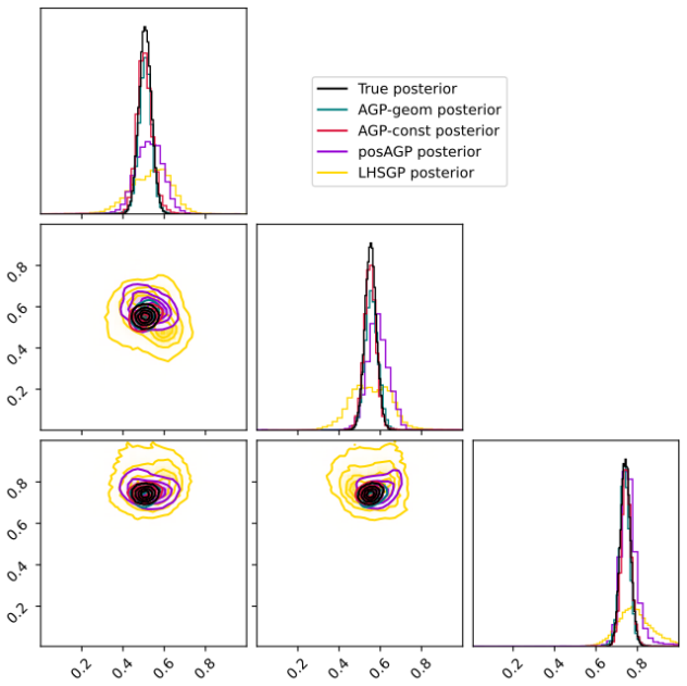
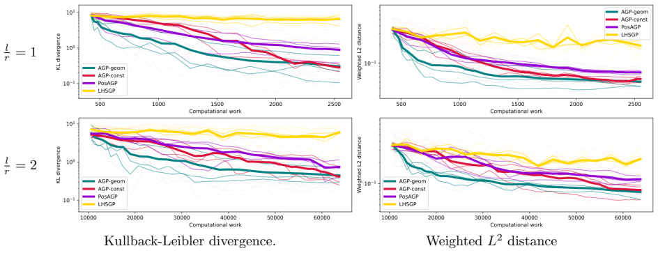
The paper's central discovery is a working formulation of this interleaved idea: it converts the unknown error between the true posterior and the surrogate-based posterior into computable error models, namely an upper bound on the Kullback-Leibler divergence (Theorem 1, Eq. (13)) and a posterior-weighted $L^2$ error model (Eq. (14)), and then uses these to drive a sequential greedy design. At each iteration, MCMC samples from the current surrogate-based posterior weight the acquisition function (20) that scores candidate evaluation points, and the same samples discretize the tolerance optimization problem (21) that reallocates the remaining budget among old and new points. The paper shows numerically that this joint adaptation beats position-only adaptation, that tolerance optimization is most valuable when more accurate solves are cheap relative to the work model $W(\tau)=\tau^{-l/r}$, and that the fully adaptive designs end with far fewer training points, so both forward evaluations and surrogate evaluations become cheaper.
Load-bearing premise
Everything hinges on the assumption that a forward-model evaluation with tolerance $\tau$ returns the true value plus independent zero-mean Gaussian noise with standard deviation $\tau$; real discretization errors from adaptive solvers are not independent or Gaussian, and the numerical experiments substitute Gaussian noise for actual solver error.
Editorial extensions
If this is right
- Under the paper's error model, tolerance optimization plus position adaptation converges to the target posterior with fewer forward-model evaluations than position-only or static designs on the same budget.
- Tolerance optimization pays off most when the work model exponent $l/r$ is small, i.e. when increasing evaluation accuracy is comparatively cheap; for expensive accurate solves, position adaptation nearly suffices.
- Fully adaptive designs end with substantially fewer training points, making the surrogate itself cheaper to evaluate during sampling.
- Using the stochastic likelihood (6) instead of plugging in the GP mean guards against overconfident posteriors in early iterations.
- Reusing samples in a sliding window reduces sampling cost when the posterior changes little between iterations.
Reading between the lines
- Because the experiments emulate discretization error as independent zero-mean Gaussian noise with variance $\tau^2$, the reported efficiency gains are best read as an upper bound for real adaptive PDE solvers, whose discretization errors are correlated and not Gaussian; the acquisition rule may misallocate budget in that regime.
- Tolerance re-optimization assumes evaluations can be stored and continued from previous grids; for black-box solvers that cannot resume a solve, the method loses much of its advantage even if the error model held.
- A natural testable extension is to treat the reported tolerance $\tau_i$ as a tunable hyperparameter or to model correlated error components, and to compare the greedy acquisition (20) against a fully Bayesian design under the same budget.
- The bound (13) sets $\alpha=1$ optimistically once the surrogate is reasonable, so in early iterations the true bound may be larger and practical convergence could depend on the initial design more than the asymptotic analysis suggests.
Editorial analysis
A structured set of objections, weighed in public.
Referee Report
Summary. This paper proposes a fully adaptive Gaussian-process surrogate strategy for sampling Bayesian posteriors. Starting from an initial design, Algorithm 1 interleaves MCMC sampling from the current surrogate-based posterior with greedy design updates: candidate evaluation points are selected as local maximizers of the acquisition function (20), and evaluation tolerances are re-optimized in (21) under a work-model constraint. Two error models are derived, the KL-divergence model (13) based on Theorem 1 and Lemma 1, and the posterior-weighted L2 model (14). Numerical experiments on a 2D synthetic example, a 3D diffusion example, and a 4D Poisson example compare AGP-const and AGP-geom with position-only-adaptive (posAGP) and static LHSGP designs, reporting improved convergence and fewer training points. The abstract's central claim is that joint optimization of positions and tolerances significantly reduces computational effort.
Significance. Strengths: the fully stochastic likelihood (6) is a principled treatment of surrogate uncertainty; Theorem 1 and Lemma 1 provide explicit, analytically derived error bounds; Appendix A gives closed-form derivatives, making the acquisition and tolerance optimization concrete and reproducible; the experimental matrix across dimensions, cost models, and error metrics is extensive. If the observed gains survive contact with genuine adaptively-refined PDE solvers, the method would be a practical improvement over position-only-adaptive surrogates. However, the current numerical evidence is produced under the Gaussian-noise idealization of Section 3.1, not under the FE discretization errors the method is motivated by, so the significance for the intended application is not yet established.
major comments (4)
- [5.1; Remark 1] The central numerical claim in the abstract, that jointly optimizing evaluation positions and tolerances yields a significant reduction of computational effort, is supported only under the idealized error model of Section 3.1, in which evaluation errors are independent N(0, tau_i^2) draws. Section 5.1 implements this by adding Gaussian noise to analytic forward models; no actual adaptive FE solver is run. Because FE discretization errors are deterministic, generally biased, and spatially correlated (as Remark 1 concedes), the tolerance-optimization steps in (18) and (21) use the wrong likelihood for the intended application. A concrete test would be to run Algorithm 1 with an actual adaptive FE solve, or with a deterministic error model having known, correlated error, and to report whether the observed reduction over posAGP and LHSGP persists; without such a test the abstract's claim is overstated.
- [4.1.1, Eq. (13)] Theorem 1 assumes pi_D(y_m) <= alpha pi(y_m) for some finite alpha, but the error model sets log alpha = 0 'optimistically'. Since L_D(p) is the convolution of the measurement error with the GP predictive density, the evidence ratio pi_D(y_m)/pi(y_m) is not generally bounded by 1, especially when the surrogate mean is biased. Dropping log alpha systematically underestimates e^KL_D(p) and can change the selected positions and tolerances in (20) and (21). The authors should either justify alpha = 1 from the setting, estimate the ratio, or report the sensitivity of the resulting designs to the value of log alpha.
- [5.2-5.4, Eq. (15)] The work model W(tau) = tau^{-l/r} is assumed and not measured, and the reported savings are expressed in units of this assumed model rather than in wall-clock time or actual solver effort. Table 1 and Table 2 report numbers of training points, but the adaptive strategies also spend computational effort on multi-start optimization for (20), SLSQP for (21), and MCMC sampling between iterations; this overhead is not included in the comparison. To substantiate the claimed reduction in computational effort, the paper should report the overhead of the design optimization and, ideally, total runtime for each strategy.
- [4.3.1, Eq. (18)] The acquisition function and the tolerance optimization in (19) replace the posterior pi(.|y_m,D_j) by the currently available pi(.|y_m,D_{j-1}) and freeze the predictive mean at the previous iterate. These substitutions are acknowledged, but they are not covered by Theorem 1, so the resulting error model is an ad-hoc heuristic whose failure modes are not assessed. The numerical section should include a sensitivity check, for example comparing the designs produced by the heuristic against a small number of random design perturbations, or against an oracle that evaluates (8) with the exact posterior, to show that the design decisions are robust to this approximation.
minor comments (4)
- [3.1] The sentence 'Gaussian process Regression (GPR) is an approximation technique that can efficiently learn large classes of functions [23], providing a .' contains an incomplete final phrase; the missing object should be supplied.
- [Algorithm 1, step 3] The notation r_j is used before it is defined, and the final design is written as D_j = ((p_i,tau_i))_{i=1,...,s_j+1}, which does not clearly account for candidates excluded by tau_i = infinity; please clarify the indexing.
- [Figures 5, 6, 10] The convergence plots do not label their axes; please state explicitly whether the horizontal axis is iteration number or accumulated work and what the vertical metric is (e.g., E^KL or E^{L2}).
- [References] Reference [30] is cited only as 'In Proceedings Of The Conference Algoritmy, 2024'; please provide complete bibliographic information.
Circularity Check
No significant circularity: the efficiency claim is a new empirical comparison conditional on an explicitly stated idealized error model; prior self-citations are contextual, not load-bearing.
full rationale
The derivation chain is self-contained rather than circular. The error models (13) and (14) are GP-averaged upper bounds derived in Theorem 1, Lemma 1 and Corollaries 1-2; although they are evaluated with the current surrogate posterior and predictive variance Gamma(p), they serve only as acquisition and tolerance-selection heuristics in Algorithm 1 (Eqs. (20)-(21)), while the reported convergence rates are measured as actual errors against the analytically available forward models (Sec. 5.1), so the central claim is not identical to the optimized surrogate objective. The method extends the authors' earlier work [30], and the acquisition rule cites [30, 26], but the algorithm and derivative formulas are fully specified here rather than importing an unverified premise, and no uniqueness theorem or forbidden alternative is invoked. The work model W(tau)=tau^(-l/r) (Eq. (15)) is an assigned asymptotic model, not a fitted parameter, so no quantity is fitted and then renamed as a prediction. The paper itself flags in Remark 1 that independent Gaussian evaluation errors are 'for sure not satisfied' for FE discretization errors, and Sec. 5.1 simulates discretization error by adding Gaussian noise to analytic models; this is an explicitly acknowledged limitation affecting transferability of the efficiency claim, but it does not make any derived result equivalent to its inputs by construction.
Assumptions & free parameters
free parameters (2)
- Geometric budget ratio alpha (AGP-geom) =
1.173 (2D), 1.178 (3D), 1.148 (4D)
- Initial tolerance tau for default evaluations =
0.05 (2D), 0.02 (3D), 0.04 (4D)
assumptions (5)
- domain assumption Forward model evaluations are corrupted by independent, zero-mean Gaussian noise with standard deviation equal to the tolerance tau_i.
- domain assumption The computational cost of an evaluation depends only on the tolerance via W(tau)=tau^(-l/r).
- ad hoc to paper The ratio pi_D(y_m)/pi(y_m) is bounded by alpha, and alpha may be set to 1.
- standard math The forward model y is a realization of a Gaussian process GP(mu,k) with known kernel.
- domain assumption Evaluation results can be stored and refined, and grids can be reused across parameter points.
Cite this review
Pith. "Pith review of Posterior sampling with Adaptive Gaussian Processes in Bayesian parameter identification." pith.science (2026). https://pith.science/paper/Q5IIPZVO
@misc{pith2026241117858,
  author       = {Pith},
  title        = {Pith review of: Posterior sampling with Adaptive Gaussian Processes in Bayesian parameter identification},
  year         = {2026},
  howpublished = {\url{https://pith.science/paper/Q5IIPZVO}},
  note         = {Machine review of arXiv:2411.17858}
}
read the original abstract
Posterior sampling by Monte Carlo methods provides a more comprehensive solution approach to inverse problems than computing point estimates such as the maximum posterior using optimization methods, at the expense of usually requiring many more evaluations of the forward model. Replacing computationally expensive forward models by fast surrogate models is an attractive option. However, computing the simulated training data for building a sufficiently accurate surrogate model can be computationally expensive in itself, leading to the design of computer experiments problem of finding evaluation points and accuracies such that the highest accuracy is obtained given a fixed computational budget. Here, we consider a fully adaptive greedy approach to this problem. Using Gaussian process regression as surrogate, samples are drawn from the available posterior approximation while designs are incrementally defined by solving a sequence of optimization problems for evaluation accuracy and positions. The selection of training designs is tailored towards representing the posterior to be sampled as good as possible, while the interleaved sampling steps discard old inaccurate samples in favor of new, more accurate ones. Numerical results show a significant reduction of the computational effort compared to just position-adaptive and static designs.
Figures


Figures from the paper (7 more)




Forward citations
Cited by 1 Pith paper
-
Robust Surrogate-Based Bayesian Inference via Sampling-Based Adaptive Active Learning (SALE)
Using the expected posterior as a common design measure for both optimization and uncertainty reduction yields robust finite-budget posterior approximations.
Reference graph
Works this paper leans on
-
[1]
T. Bai, A. L. Teckentrup, and K. C. Zygalakis. Gaussian processes for bayesian inverse problems associated with linear partial differential equations. Statistics and Computing , 34, 2024
work page 2024
-
[2]
G. Boehl. An ensemble mcmc sampler for robust bayesian inference. Technical report, University of Bonn, 2024
work page 2024
-
[3]
J. A. Christen and C. Fox. Markov chain monte carlo using an approximation. Journal of Computational and Graphical Statistics , 14(4):795–810, 2005
work page 2005
-
[4]
A. Christmann and I. Steinwart. Support Vector Machines. Springer New York, NY, 2008
work page 2008
-
[5]
K. Crombecq, E. Laermans, and T. Dhaene. Efficient space-filling and non-collapsing sequential design strategies for simulation-based modeling. European Journal of Operational Research , 214:683–696, 2011
work page 2011
- [6]
-
[7]
D. K. Duvenaud. Automatic Model Construction with Gaussian Processes . Phd thesis, Univer- sity of Cambridge, 2014
work page 2014
-
[8]
H.W. Engl, M. Hanke, and A. Neubauer. Regularization of inverse problems . Kluwer, 1996. 20
work page 1996
Show all 36 references
-
[9]
Foreman-Mackey
D. Foreman-Mackey. corner.py: Scatterplot matrices in python. The Journal of Open Source Software, 1(2):24, jun 2016
2016
-
[10]
Foreman-Mackey, D
D. Foreman-Mackey, D. W. Hogg, D. Lang, and J. Goodman. emcee: The mcmc hammer. PASP, 125:306–312, 2013
2013
-
[11]
Gpy- torch: Blackbox matrix-matrix gaussian process inference with gpu acceleration
Jacob Gardner, Geoff Pleiss, Kilian Q Weinberger, David Bindel, and Andrew G Wilson. Gpy- torch: Blackbox matrix-matrix gaussian process inference with gpu acceleration. In S. Bengio, H. Wallach, H. Larochelle, K. Grauman, N. Cesa-Bianchi, and R. Garnett, editors, Advances in ...
2018
-
[12]
Giunta, S
A. Giunta, S. Wojtkiewicz, and M. Eldred. Overview of modern design of experiments methods for computational simulations. In 41st Aerospace Sciences Meeting and Exhibit, AIAA 2003- 649, pages 1–17, 2003
2003
-
[13]
Goodman and J
J. Goodman and J. Weare. Ensemble samplers with affine invariance. Communications in applied mathematics and computational science , 5(1):65–80, 2010
2010
-
[14]
Hastings
W.K. Hastings. Monte Carlo sampling methods using Markov chains and their applications. Biometrika, 57(1):97–109, 1970
1970
-
[15]
Helin, A.M
T. Helin, A.M. Stuart, A.L. Teckentrup, and K.C. Zygalakis. Introduction to gaussian process regression in bayesian inverse problems, with new results on experimental design for weighted error measures. In Monte Carlo and Quasi-Monte Carlo Methods , 2023
2023
-
[16]
Hennig and C.J
P. Hennig and C.J. Schuler. Entropy search for information-efficient global optimization.Journal of Machine Learning Research, 13:1809–1837, 2012
2012
-
[17]
Joseph and Y
V. Joseph and Y. Hung. Orthogonal-maximin latin hypercube designs. Statistica Sinica, 18:171– 186, 2008
2008
-
[18]
J¨ arvenp¨ a¨ a, M
M. J¨ arvenp¨ a¨ a, M. U. Gutmann, A. Vehtari, and P. Marttine. Parallel Gaussian process surrogate Bayesian inference with noisy likelihood evaluations. Bayesian Analysis, 16, pp. 147–178. , 2021
2021
-
[19]
Kaipio and E
J. Kaipio and E. Somersalo. Statistical and Computational Inverse Problems . Springer, 2005
2005
-
[20]
Lehmensiek, P
R. Lehmensiek, P. Meyer, and M. M¨ uller. Adaptive sampling applied to multivariate, multi- ple output rational interpolation models with application to microwave circuits. International Journal of RF and Microwave Computer-Aided Engineering , 12(4):332–340, 2002
2002
-
[21]
Moˇ ckus
J. Moˇ ckus. On Bayesian methods for seeking the extremum. In Optimization Techniques IFIP Technical Conference Novosibirsk, pages 400–404. Springer, 1975
1975
-
[22]
Queipo, R
N. Queipo, R. Haftka, W. Shyy, T. Goel, R. Vaidyanathan, and P. Tucker. Surrogate-based analysis and optimization. Progress in Aerospace Sciences, 41(1):1–28, 2005
2005
-
[23]
Rasmussen and C.K.I
C. Rasmussen and C.K.I. Williams. Gaussian Processes for Machine Learning . MIT Press, 2006
2006
-
[24]
Schneider, M
P. Schneider, M. Hammerschmidt, L. Zschiedrich, and S. Burger. Using Gaussian process regression for efficient parameter reconstruction. In Metrology, Inspection, and Process Control for Microlithography XXXIII, volume 10959. SPIE, 2019
2019
-
[25]
Semler and M
P. Semler and M. Weiser. Adaptive Gaussian process regression for efficient building of surrogate models in inverse problems. Inverse Problems, 39:125003, 2023
2023
-
[26]
Semler and M
P. Semler and M. Weiser. Adaptive gradient enhanced gaussian process surrogates for inverse problems. In Proceedings of the MATH+ Thematic Einstein Semester 2023 , 2024
2023
-
[27]
Sinsbeck and W
M. Sinsbeck and W. Nowak. Sequential design of computer experiments for the solution of bayesian inverse problems. SIAM/ASA Journal on Uncertainty Quantification , 5(1):640–664, 2017. 21
2017
-
[28]
Sugiyama
M. Sugiyama. Active learning in approximately linear regression based on conditional expecta- tion of generalization error. Journal of Machine Learning Research , 7:141––166, 2006
2006
-
[29]
Ter Braak
C.J.F. Ter Braak. A markov chain monte carlo version of the genetic algorithm differential evolu- tion: easy bayesian computing for real parameter spaces. Statistics and Computing, 16:239–249, 2006
2006
-
[30]
Villani, J
P. Villani, J. F. Unger, and M. Weiser. Adaptive gaussian process regression for bayesian inverse problems. In Proceedings Of The Conference Algoritmy, 2024
2024
-
[31]
Wang and M
Z. Wang and M. Broccardo. A novel active learning-based gaussian process metamodelling strategy for estimating the full probability distribution in forward uq analysis. Struct. Safety , 84:101937, 2020
2020
-
[32]
Weiser and S
M. Weiser and S. Ghosh. Theoretically optimal inexact spectral deferred correction methods. Commu. Appl. Math. Comp. Sci. , 13(1):53–86, 2018
2018
-
[33]
J. Wu, M. Poloczek, A.G. Wilson, and P.I. Frazier. Bayesian optimization with gradients. In Advances in Neural Information Processing Systems , volume 30, pages 3–6. Curran Associates, 2017
2017
-
[34]
A. Zaytsev. Reliable surrogate modeling of engineering data with more than two levels of fidelity. In 2016 7th International Conference on Mechanical and Aerospace Engineering (ICMAE) , pages 341–345, 2016
2016
-
[35]
H. Zhu, R. H. Byrd, and J. Nocedal. Algorithm 778: L-bfgs-b, fortran routines for large scale bound constrained optimization. ACM Transactions on Mathematical Software , 23:550–560, 1997
1997
-
[36]
´Alvarez, L
M.A. ´Alvarez, L. Rosasco, and N.D. Lawrence. Kernels for vector-valued functions: A review. Foundations and Trends in Machine Learning , 4(3):195–266, 2012. A Target function derivatives This appendix contains the analytical expression of the derivatives contained in the acqu...
2012
Reviewed August 12, 2026 · model on record in the stance chip above.
Discussion (0). Continue with ORCID to comment.