REVIEW 3 major objections 6 minor 51 references
Quantifying Suppression of Solar Surface Magnetic Flux Advection with Increasing Field Strength
T0 review · 3 major / 6 minor · reviewed 2026-08-15 · deepseek-v4-flash
Pith's one-line read The Sun's magnetic flux advection slows from 110 to 10 m/s as vertical field strength rises from 150 to 2500 G.
desk verdict A solid, well-documented first uniform measurement of flux advection suppression, but the headline polynomial's absolute speeds are cadence- and kernel-dependent and need a noise-floor calibration before use in MHD models. read the letter →
The pith
A machine-rendered reading of the paper's core claim, the machinery that carries it, and where it could break.
The reading
What carries the argument
The central tool is Fourier Local Correlation Tracking (FLCT), applied to 12-minute-cadence HMI SHARP Bz magnetograms. FLCT measures the horizontal displacement of magnetic-flux patterns between consecutive frames by cross-correlating Gaussian-weighted subimages (here with a 15-pixel FWHM kernel spanning ~5.4 Mm, about five granules), then converts the displacement into a speed. The argument is carried by binning measured speeds in 50 G-wide Bz bins, averaging over 24 hours per active region, and fitting the mean curve with a fourth-degree polynomial. The Bz threshold of 150 G (~2σ noise) defines the weak-field endpoint, and the choice of Bz rather than BLOS or |B_total| is justified by lower noise and by Bz being the vertical magnetic flux density.
What would settle it
Re-run the FLCT analysis on the same magnetograms but with a 9-pixel or 6-pixel kernel and with 6-minute cadence; if the mean speeds at 150-200 G do not stay within the reported 110 ± 3 m/s, or if the curve's shape changes materially, the specific polynomial is an artifact of the kernel and cadence choices rather than a robust physical relation.
Extended reading notes
Core claim
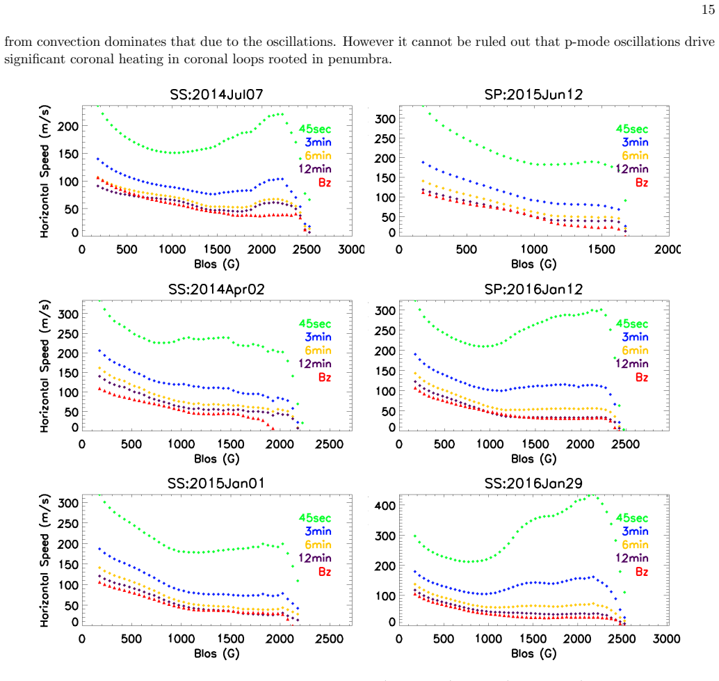
The paper reports that horizontal advection of magnetic flux, measured with FLCT on 12-minute-cadence HMI SHARP Bz magnetograms of six non-flaring active regions, decreases monotonically with increasing vertical field strength Bz. Mean speeds fall from 110 ± 3 m/s in the 150–200 G bin (network and plage) to 10 ± 4 m/s in the 2400–2500 G bin (sunspot umbra), with a plateau near 1200–2000 G and a slight bump before the drop to near-zero speeds at the strongest fields. The combined mean is fit by $v_h = -1.55\times10^{-14} x^4 + 7.06\times10^{-11} x^3 - 7.97\times10^{-8} x^2 - 3.92\times10^{-5} x + 0.11$ (km/s), where $x$ is Bz in G. The authors take this as quantitative confirmation that stronger magnetic fields increasingly suppress convection-driven flux advection, and as the first uniform measurement of that suppression across network, plage, penumbra, and umbra.
Load-bearing premise
The entire quantitative relation rests on the assumption that the motions FLCT measures in Bz maps at 12-minute cadence with a 15-pixel kernel are the true horizontal advection speeds of magnetic flux driven by convection, accurate even at the ~10 m/s level where the per-frame displacement is only ~0.02 pixels.
Editorial extensions
If this is right
- The empirical curve gives magneto-convection and coronal heating simulations a direct boundary condition: how fast photospheric footpoints are shuffled as a function of local field strength.
- The relation can be folded into coronal loop heating scaling laws to include loops rooted in sunspot umbrae, which current field-strength-and-length laws fail to fit.
- The monotonic decrease quantitatively confirms and extends the earlier plage-only trend of Title et al. (1992) to the full range from network to umbra.
- The plateau and the bump near the penumbra-umbra boundary, if real, point to additional velocity contributions (penumbral filaments, moat flows, possible p-mode oscillations) that are not pure advection.
Reading between the lines
- Because FLCT with a 15-pixel kernel averages over scales of ~5 granules, Eq. (1) should be read as a mesogranular-scale advection law; granular-scale advection of weak flux may be considerably faster, and testing the same method at higher spatial resolution could yield a steeper curve at the weak-field end.
- At 2500 G the measured 10 ± 4 m/s is comparable to the expected tracking noise for 12-minute cadence, so the strong-field end of the curve may represent an upper bound on umbral advection rather than a resolved value.
- The polynomial fit is empirical; a physically motivated form (e.g., advection speed scaling with the ratio of magnetic to gas pressure) could be fitted to the binned means and compared, which would test whether the plateau and bump have dynamical meaning.
Signed reviews
Editorial analysis
A structured set of objections, weighed in public.
Referee Report
Summary. The paper measures the horizontal advection speed of magnetic flux as a function of vertical field strength (Bz) in six active regions using Fourier Local Correlation Tracking (FLCT) on HMI SHARP Bz magnetograms at 12-minute cadence. The authors report a monotonic decrease in the average advection speed from about 110 m/s at 150 G to about 10 m/s at 2500 G, fit a fourth-degree polynomial (Eq. 1), and compare results with BLOS magnetograms at several cadences. They interpret the trend as quantitative confirmation that strong magnetic fields suppress convective advection of flux and propose the relation as an empirical input for future MHD models of coronal heating.
Significance. If the quantitative relation were well calibrated, this would be the first uniform measurement of flux advection speed across the full range from network/plage to sunspot umbrae, and it would provide a useful empirical input for coronal heating models. Strengths of the study include the use of six stable, non-flaring active regions, consistent data processing, and cross-checks against BLOS data at multiple cadences and against earlier results (Title et al. 1992; Sobotka et al. 2012). The qualitative trend—decreasing speed with increasing field strength—is robust across all six ARs and agrees with prior work. However, the absolute speed scale and therefore the polynomial in Eq. (1) are not yet established as physical, owing to the missing calibration of FLCT at sub-pixel displacements and the known cadence and temporal-smoothing dependencies.
major comments (3)
- [Section 2.2, Eq. (1)] The paper provides no noise-floor or minimum-detectable-velocity analysis for FLCT. At the stated CEA scale of 360 km/pixel and 12-minute cadence, the quoted 10 m/s at 2500 G corresponds to a displacement of about 0.02 pixels per frame, and even 110 m/s at 150 G is only 0.22 pixels. Without synthetic tests or calibration against known displacements, the absolute speeds in Eq. (1) and in the abstract (110 ± 3 and 10 ± 4 m/s) cannot be taken as physical advection speeds; the error bars in Figs. 3 and 6 are spreads of the data, not tracking uncertainties. Since Eq. (1) is the central quantitative result, this gap is load-bearing.
- [Section 4, Fig. 9] The authors' own comparison shows that 45-second BLOS speeds are two to three times larger than 12-minute Bz speeds, and Section 2.2 states that the 15-pixel kernel was chosen by visual persistence rather than calibration. Because the paper claims in Section 1 to 'establish a general relation,' Eq. (1) as presented is not invariant to the measurement settings. The paper should either calibrate the speeds to make them independent of cadence and kernel, or explicitly present Eq. (1) as a measurement-specific relation with clear caveats about how the absolute values would change.
- [Appendix .1] The Bz magnetograms used in the main analysis are temporally averaged with a 1215-second boxcar and a cosine weighting function with an FWHM of 720 seconds. This smoothing is likely to suppress short-lived motions and bias the measured 12-minute velocities downward. The paper does not quantify this bias or its impact on Eq. (1). Because the main analysis is based on these smoothed maps, the polynomial in Eq. (1) may underestimate the true horizontal advection speed even at 12-minute cadence.
minor comments (6)
- [Section 2.2] The acronym 'FCLT' should be 'FLCT', and 'Guassian' should be 'Gaussian'.
- [Figure 3 caption] The red error bars, described as standard error, are mostly hidden inside the diamond markers; consider using caps or a different marker style so that the small standard errors are visible to the reader.
- [Section 3.3, Fig. 7] The figure caption should explicitly state that the blue error bars are divided by four for display, rather than leaving this information only in the main text.
- [Appendix headings] The appendix headings appear as '.1' and '.2' instead of 'A.1' and 'A.2'; please fix the formatting.
- [Table 1] The 'Max Flare' entry for AR 12108 is '–'; using 'None' would be consistent with the text and clearer to readers.
- [Eq. (1)] Reporting uncertainties for the polynomial coefficients would allow readers to assess the fit quality and would strengthen the quantitative claim.
Circularity Check
No circularity: the speed-versus-Bz relation is an empirical fit to measured FLCT speeds, and self-citations are only motivational.
full rationale
The paper's central result is an empirical trend obtained by applying FLCT (Fisher & Welsch 2008) to HMI SHARP Bz magnetograms and averaging measured horizontal speeds in 50 G bins of Bz, then fitting a fourth-degree polynomial to the binned means (Eq. 1). The independent variable Bz is the field strength at each pixel and the dependent variable is the temporal displacement-derived speed; neither is defined in terms of the other, and no fitted parameter is used to construct the input magnetograms or velocities. The polynomial is explicitly a fit to the measured means, not a prediction derived from the fit. The self-cited prior work (Tiwari et al. 2017) motivates the coronal-heating context but does not enter the measurement or the fit; the method citation Fisher & Welsch (2008) supplies an external, public algorithm rather than an unverified premise. Comparisons with Title et al. (1992), Sobotka et al. (2012), and the paper's own BLOS/cadence checks provide independent context. Concerns about FLCT's noise floor or the dependence of absolute speeds on cadence and kernel are calibration and correctness issues, not circularity, because they do not make the output equal to an input by construction.
Assumptions & free parameters
free parameters (3)
- Polynomial coefficients a0-a4 (Eq. 1) =
0.11, -3.92e-5, -7.97e-8, 7.06e-11, -1.55e-14
- FLCT Gaussian kernel FWHM =
15 pixels, about 5.4 Mm
- Bz threshold for tracking =
150 G
assumptions (4)
- domain assumption Horizontal advection of flux is driven by horizontal convective plasma flows.
- domain assumption FLCT speeds of Bz patterns at 12-minute cadence with a 15-pixel kernel are accurate at the ~10 m/s level.
- domain assumption The six selected active regions are representative of the solar surface field strength range from 150 to 2500 G.
- domain assumption SHARP CEA Bz data have about 70 G noise, so a 150 G threshold is a safe detection limit.
Cite this review
Pith. "Pith review of Quantifying Suppression of Solar Surface Magnetic Flux Advection with Increasing Field Strength." pith.science (2026). https://pith.science/paper/QB7DWXH5
@misc{pith2026250504511,
  author       = {Pith},
  title        = {Pith review of: Quantifying Suppression of Solar Surface Magnetic Flux Advection with Increasing Field Strength},
  year         = {2026},
  howpublished = {\url{https://pith.science/paper/QB7DWXH5}},
  note         = {Machine review of arXiv:2505.04511}
}
read the original abstract
One of the main theories for heating of the solar corona is based on the idea that solar convection shuffles and tangles magnetic field lines to make many small-scale current sheets that, via reconnection, heat coronal loops. Tiwari et al 2017 present evidence that, besides depending on loop length and other factors, the brightness of a coronal loop depends on the field strength in the loop feet and the freedom of convection in the feet. While it is known that strong solar magnetic fields suppress convection, the decrease in the speed of horizontal advection of magnetic flux with increasing field strength has not been quantified before. We quantify that trend by analyzing 24hours of HMI SHARP vector magnetograms of each of six sunspot active regions and their surroundings. Using Fourier Local Correlation Tracking, we estimate the horizontal advection speed of the magnetic flux at each pixel in which the vertical component of the magnetic field strength (Bz) is well above (greater than or equal to 150 G) noise level. We find that the average horizontal advection speed of magnetic flux steadily decreases as Bz increases, from 110 pm 3 meters per sec for 150 G (in network and plage) to 10 pm 4 meters per sec for 2500 G (in sunspot umbra). The trend is well fit by a fourth degree polynomial. These results quantitatively confirm the expectation that magnetic flux advection is suppressed by increasing magnetic field strength. The presented quantitative relation should be useful for future MHD simulations of coronal heating.
Figures


Figures from the paper (8 more)




Reference graph
Works this paper leans on
-
[1]
Archontis, V., & Syntelis, P. 2019, Philosophical Transactions of the Royal Society of London Series A, 377, 20180387, doi: 10.1098/rsta.2018.0387
arXiv 2019
-
[2]
Bahauddin, S. M., Bradshaw, S. J., & Winebarger, A. R. 2021, Nature Astronomy, 5, 237, doi: 10.1038/s41550-020-01263-2
-
[3]
Beckers, J. M. 1977, ApJ, 213, 900, doi: 10.1086/155222
doi:10.1086/155222 1977
-
[4]
Scherrer, P. H., & Slater, G. L. 2002, ApJL, 571, L181, doi: 10.1086/341203
-
[5]
Bobra, M. G., Sun, X., Hoeksema, J. T., et al. 2014, SoPh, 289, 3549, doi: 10.1007/s11207-014-0529-3
-
[6]
Brown, T. M., Bogdan, T. J., Lites, B. W., & Thomas, J. H. 1992, ApJL, 394, L65, doi: 10.1086/186473
-
[7]
Weiss, N. O. 2008, MNRAS, 387, 698, doi: 10.1111/j.1365-2966.2008.13276.x
arXiv 2008
-
[8]
2006, SoPh, 236, 415, doi: 10.1007/s11207-006-0103-8
Cavallini, F. 2006, SoPh, 236, 415, doi: 10.1007/s11207-006-0103-8
Show all 51 references
-
[9]
A., et al
Couvidat, S., Schou, J., Shine, R. A., et al. 2012, SoPh, 275, 285, doi: 10.1007/s11207-011-9723-8 De Pontieu, B., Erd´ elyi, R., & James, S. P. 2004, Nature, 430, 536, doi: 10.1038/nature02749 De Rosa, M., Duvall, T. L., J., & Toomre, J. 2000, SoPh, 192, 351, doi: 10.1023/A:1...
2012 doi
-
[10]
A., Tiwari, S
Falconer, D. A., Tiwari, S. K., Moore, R. L., & Khazanov, I. 2016, ApJL, 833, L31, doi: 10.3847/2041-8213/833/2/L31
2016 doi
- [11]
-
[12]
Gosain, S., Venkatakrishnan, P., & Tiwari, S. K. 2009, ApJL, 706, L240, doi: 10.1088/0004-637X/706/2/L240
2009 doi
-
[13]
H., Beck, J
Hathaway, D. H., Beck, J. G., Bogart, R. S., et al. 2000, SoPh, 193, 299, doi: 10.1023/A:1005200809766 Hinode Review Team, Al-Janabi, K., Antolin, P., et al. 2019, PASJ, 71, R1, doi: 10.1093/pasj/psz084
2000 doi
-
[14]
T., Liu, Y., Hayashi, K., et al
Hoeksema, J. T., Liu, Y., Hayashi, K., et al. 2014, SoPh, 289, 3483, doi: 10.1007/s11207-014-0516-8
2014 doi
-
[15]
B., Rempel, M., et al
Kilcik, A., Yurchyshyn, V. B., Rempel, M., et al. 2012, ApJ, 745, 163, doi: 10.1088/0004-637X/745/2/163
2012 doi
-
[16]
2020, A&A, 633, A67, doi: 10.1051/0004-6361/201936778 Kors´ os, M
Kontogiannis, I., Tsiropoula, G., Tziotziou, K., et al. 2020, A&A, 633, A67, doi: 10.1051/0004-6361/201936778 Kors´ os, M. B., Romano, P., Morgan, H., et al. 2020, ApJL, 897, L23, doi: 10.3847/2041-8213/ab9d7a
2020 doi
-
[17]
M., Roudier, T., & Rieutord, M
Krijger, J. M., Roudier, T., & Rieutord, M. 2002, A&A, 387, 672, doi: 10.1051/0004-6361:20020405
2002 doi
-
[18]
D., Barnes, G., Crouch, A
Leka, K. D., Barnes, G., Crouch, A. D., et al. 2009, SoPh, 260, 83, doi: 10.1007/s11207-009-9440-8
2009 doi
-
[19]
2019, ApJ, 876, 129, doi: 10.3847/1538-4357/ab18aa
Li, Q., Deng, N., Jing, J., Liu, C., & Wang, H. 2019, ApJ, 876, 129, doi: 10.3847/1538-4357/ab18aa
2019 doi
-
[20]
Liu, Y., Zhao, J., & Schuck, P. W. 2013, SoPh, 287, 279, doi: 10.1007/s11207-012-0089-3
2013 doi
-
[21]
T., Scherrer, P
Liu, Y., Hoeksema, J. T., Scherrer, P. H., et al. 2012, SoPh, 279, 295, doi: 10.1007/s11207-012-9976-x
2012 doi
-
[22]
S., & Hanasoge, S
Mani, P., Hanson, C. S., & Hanasoge, S. 2022, ApJ, 926, 127, doi: 10.3847/1538-4357/ac474e
2022 doi
-
[23]
W., & Jefferies, S
McIntosh, S. W., & Jefferies, S. M. 2006, ApJL, 647, L77, doi: 10.1086/507425 Nordlund, ˚A., Stein, R. F., & Asplund, M. 2009, Living Reviews in Solar Physics, 6, 2, doi: 10.12942/lrsp-2009-2
2006 doi
- [24]
-
[25]
S., Tofani, G., & Felli, M
Pallavicini, R., Vaiana, G. S., Tofani, G., & Felli, M. 1979, ApJ, 229, 375, doi: 10.1086/156963
1979 doi
-
[26]
H., & Haywood, R
Palumbo, Michael L., I., Saar, S. H., & Haywood, R. D. 2024, ApJ, 973, 11, doi: 10.3847/1538-4357/ad445a
2024 doi
-
[27]
Parker, E. N. 1988, ApJ, 330, 474, doi: 10.1086/166485
1988 doi
-
[28]
D., Thompson, B
Pesnell, W. D., Thompson, B. J., & Chamberlin, P. C. 2012, SoPh, 275, 3, doi: 10.1007/s11207-011-9841-3
2012 doi
-
[29]
2011, ApJ, 729, 5, doi: 10.1088/0004-637X/729/1/5
Rempel, M. 2011, ApJ, 729, 5, doi: 10.1088/0004-637X/729/1/5
2011 doi
-
[30]
2011, Living Reviews in Solar Physics, 8, 3, doi: 10.12942/lrsp-2011-3
Rempel, M., & Schlichenmaier, R. 2011, Living Reviews in Solar Physics, 8, 3, doi: 10.12942/lrsp-2011-3
2011 doi
-
[31]
2018, Living Reviews in Solar Physics, 15, 6, doi: 10.1007/s41116-018-0013-5
Rincon, F., & Rieutord, M. 2018, Living Reviews in Solar Physics, 15, 6, doi: 10.1007/s41116-018-0013-5
2018 doi
-
[32]
H., Schou, J., Bush, R
Scherrer, P. H., Schou, J., Bush, R. I., et al. 2012, SoPh, 275, 207, doi: 10.1007/s11207-011-9834-2
2012 doi
-
[33]
Schuck, P. W. 2008, ApJ, 683, 1134, doi: 10.1086/589434
2008 doi
-
[34]
A., Simon, G
Shine, R. A., Simon, G. W., & Hurlburt, N. E. 2000, SoPh, 193, 313, doi: 10.1023/A:1005207625696
2000 doi
-
[35]
W., Title, A
Simon, G. W., Title, A. M., Topka, K. P., et al. 1988, ApJ, 327, 964, doi: 10.1086/166253
1988 doi
-
[36]
2012, A&A, 537, A85, doi: 10.1051/0004-6361/201117851
Sobotka, M., Del Moro, D., Jurˇ c´ ak, J., & Berrilli, F. 2012, A&A, 537, A85, doi: 10.1051/0004-6361/201117851
2012 doi
-
[37]
Sobotka, M., & Puschmann, K. G. 2022, A&A, 662, A13, doi: 10.1051/0004-6361/202243577
2022 doi
-
[38]
2007, A&A, 472, 277, doi: 10.1051/0004-6361:20077552
Sobotka, M., & Roudier, T. 2007, A&A, 472, 277, doi: 10.1051/0004-6361:20077552
2007 doi
-
[39]
Stein, R. F. 2012, Living Reviews in Solar Physics, 9, 4, doi: 10.12942/lrsp-2012-4
2012 doi
- [40]
-
[41]
M., Tarbell, T
Title, A. M., Tarbell, T. D., Topka, K. P., et al. 1989, ApJ, 336, 475, doi: 10.1086/167026 18
1989 doi
-
[42]
M., Topka, K
Title, A. M., Topka, K. P., Tarbell, T. D., et al. 1992, ApJ, 393, 782, doi: 10.1086/171545
1992 doi
-
[43]
K., Thalmann, J
Tiwari, S. K., Thalmann, J. K., Panesar, N. K., Moore, R. L., & Winebarger, A. R. 2017, ApJL, 843, L20, doi: 10.3847/2041-8213/aa794c
2017 doi
-
[44]
K., van Noort, M., Lagg, A., & Solanki, S
Tiwari, S. K., van Noort, M., Lagg, A., & Solanki, S. K. 2013, A&A, 557, A25, doi: 10.1051/0004-6361/201321391
2013 doi
-
[45]
K., van Noort, M., Solanki, S
Tiwari, S. K., van Noort, M., Solanki, S. K., & Lagg, A. 2015, A&A, 583, A119, doi: 10.1051/0004-6361/201526224
2015 doi
-
[46]
2019, ApJ, 877, 129, doi: 10.3847/1538-4357/ab1d4d van Noort, M., Lagg, A., Tiwari, S
Wiegelmann, T. 2019, ApJ, 877, 129, doi: 10.3847/1538-4357/ab1d4d van Noort, M., Lagg, A., Tiwari, S. K., & Solanki, S. K. 2013, A&A, 557, A24, doi: 10.1051/0004-6361/201321073
2019 doi
-
[47]
2009, ApJ, 702, 1048, doi: 10.1088/0004-637X/702/2/1048
Watanabe, H., Kitai, R., & Ichimoto, K. 2009, ApJ, 702, 1048, doi: 10.1088/0004-637X/702/2/1048
2009 doi
- [48]
-
[49]
T., Kusano, K., Yamamoto, T
Welsch, B. T., Kusano, K., Yamamoto, T. T., & Muglach, K. 2012, ApJ, 747, 130, doi: 10.1088/0004-637X/747/2/130
2012 doi
-
[50]
K., Woch, J., & Wang, J
Zhang, J., Solanki, S. K., Woch, J., & Wang, J. 2007, A&A, 471, 1035, doi: 10.1051/0004-6361:20077900
2007 doi
-
[51]
2024, A&A, 686, A75, doi: 10.1051/0004-6361/202348850
Zheng, C., Roudier, T., Schmieder, B., et al. 2024, A&A, 686, A75, doi: 10.1051/0004-6361/202348850
2024 doi
Reviewed August 15, 2026 · model on record in the stance chip above.
Discussion (0). Continue with ORCID to comment.