REVIEW 4 major objections 6 minor 14 references
Explainable topological data analysis using persistence heatmaps
T0 review · 4 major / 6 minor · reviewed 2026-08-04 · deepseek-v4-flash
Pith's one-line read The paper claims that averaging unstable representative cycles over random perturbations yields stable, class-revealing heatmaps—the expected persistence heatmap—with explicit Lipschitz bounds.
desk verdict Good idea, clean exposition, but the main stability theorems are stated for an undefined convolution — fix the domain issue and this becomes a credible TDA explainability tool. read the letter →
The pith
A machine-rendered reading of the paper's core claim, the machinery that carries it, and where it could break.
The reading
What carries the argument
The central objects are the annotated persistence diagram—each birth–death pair decorated with the chain (representative cycle, bounding chain, birth simplex, or death simplex) that the persistence algorithm outputs—and the persistence heatmap η that distributes each feature's weight equally over the simplices in its chain. The stabilizing mechanism is convolution: η∗K averages these chain-weights over kernel perturbations of the input, and the key inequality is the kernel's L1 displacement bound ∫|Ki(s+t)−Ki(t)|ds ≤ b_i‖t‖, which converts a small input move into a small change in the averaged output. The same convolution is applied to the composed map Θ=Π∘(η×I) that sends weights and a geom
What would settle it
Compute the heatmap image for a single edge of weight 1 whose geometric realization crosses a voxel boundary, and move one endpoint by ε so the crossing point shifts. The fraction of the edge assigned to each voxel changes with slope that depends on the edge length and grid size, and if the edge is short relative to a voxel this slope can be arbitrarily large; repeating at two grid resolutions will show the Lipschitz constant is not independent of resolution, contradicting Corollaries 5.5–5.7 as stated.
Extended reading notes
Core claim
On the paper's own terms, the discovery is that instability is not a property of the chains themselves but of choosing one chain among many equally valid ones; averaging over many perturbed inputs replaces the discrete choice with real-valued weights that vary smoothly. Concretely, for a persistence heatmap η built from the annotated chains and a kernel K with an L1 displacement bound, the expected heatmap η∗K is Lipschitz, with constants given for the three standard kernels. The same convolution argument is then applied to the composed map that projects simplices onto an image grid, yielding the claimed stable heatmaps on images whose pixel sums recover learned function values.
Load-bearing premise
The image-stability claim rests on the unproven premise that the voxel-projection map Π, which assigns each simplex's weight to grid cells by length or area fraction, is uniformly Lipschitz in the vertex coordinates; this can fail when a vertex crosses a voxel boundary or a simplex becomes degenerate, and the stated constants ignore grid resolution.
Editorial extensions
If this is right
- Representative cycles can be replaced by real-valued chain weights that change at most linearly with input perturbation, so localization maps become reliable across noise.
- Choosing the kernel radius α gives an explicit sensitivity knob: with a triangular kernel, the heatmap is 2M(k+1)√k/α-Lipschitz, so larger α smooths more.
- The visualization pipeline preserves total weight: summing pixel values recovers the total heat, which is what lets a learned regression value be reconstructed from the image.
- The construction is algorithm-agnostic: any implementation that outputs annotated persistence diagrams can feed the same stabilization.
- SVM feature coefficients can be folded into the heatmap, so the same stable image that localizes features also explains which regions push a classification one way or the other.
Reading between the lines
- The stability of the image heatmap is not actually a corollary of the chain-stability theorems: it needs a Lipschitz bound on the voxel projection Π, which the paper leaves unstated; a grid-dependent constant would change the practical guarantee.
- The same averaging recipe applies to any unstable function of the persistence diagram that is bounded and chain-valued—for example, representative cocycles or minimal generators should stabilize identically.
- Because the heatmap is a real-valued vector indexed by simplices, it can be fed into any linear model, not just SVM, so the explainability layer generalizes to logistic or ridge regression with no change to the stability proof.
Editorial analysis
A structured set of objections, weighed in public.
Referee Report
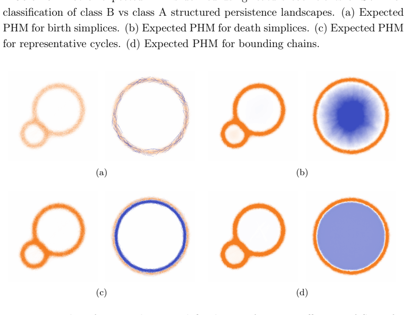
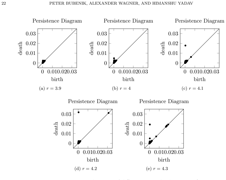
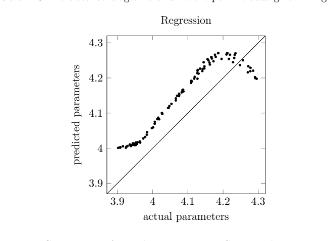
Summary. The paper introduces persistence heatmaps, a weighted-sum summary built from representative cycles, birth/death simplices, and bounding chains in annotated persistence diagrams, and proposes an “expected persistence heatmap” obtained by convolving the heatmap with a kernel. It claims uniform continuity (Theorem 1) and Lipschitz stability with explicit constants for triangular, Epanechnikov, and Gaussian kernels (Theorems 2–4, Corollaries 4.1–4.3). It further defines a visualization pipeline that maps a heatmap to a voxel grid, claims corresponding stability for the visualized heatmap (Theorem 5, Corollaries 5.5–5.7), and demonstrates SVM-based task-specific heatmaps on annular point clouds, Ginibre-ensemble eigenvalues, and linked twist maps.
Significance. If valid, the proposed persistence heatmap would give a stable, explainable TDA summary that localizes topological features in the original data space, addressing the known instability of representative cycles. The paper's theoretical framework is natural and, modulo the gaps below, the convolution-based stability arguments are standard and potentially useful. The computational examples showcase an interesting application of task-specific summaries. However, the core theoretical claims are currently undermined by an undefined convolution and an unsupported Lipschitz assumption in the visualization layer; these issues must be resolved before the paper's central promises can be accepted.
major comments (4)
- [Definition 3.2, Theorems 1–4, Corollaries 4.1–4.3] The expected persistence heatmap η∗K(x)=∫η(x−ε)K(ε)dε integrates over all R^k, but η is only defined on the monotone cone C⊂R^k. For the Gaussian kernel (Cor 4.3), supp(K)=R^k, so for every x the set {ε: x−ε∉C} has positive measure and η(x−ε) is undefined there. For compact kernels (Cor 4.1–4.2), the same issue occurs whenever B_α(x)⊄C, which is not excluded. The proofs of Theorems 1–4 integrate η over R^k, implicitly requiring an extension. Since the choice of extension alters the summary and the stability constants, the central stability results are currently statements about an undefined object. Please specify an explicit extension of η to R^k (e.g., zero, constant, or nearest-point extension) and re-state and prove the theorems under that choice.
- [Theorem 3 and Corollaries 4.1–4.2] Even if an extension is supplied, the local hypothesis “∥η∥_∞<M on B_{2α}(x)” only makes sense if B_{2α}(x) is contained in the domain on which η is actually defined. If η is defined only on C, this requires an explicit assumption that B_{2α}(x)⊆C; otherwise the convolution integral on the right-hand side is not defined. The proof uses values of η on B_α(u)∪B_α(v), which lie in C only if B_{2α}(x)⊆C. This condition is missing from the statement and from the corollaries.
- [Definition 5.3, Theorem 5, Corollaries 5.5–5.7] The claimed Lipschitz constants for Θ∗K depend only on M, k+nd, and α, and omit any dependence on grid resolution or simplex geometry. This requires the voxel-projection map Π of Definition 5.3 to be Lipschitz in the geometric-realization coordinate y with a uniform constant. The paper neither states nor proves such a bound. Π is a piecewise volume-ratio map: for a simplex σ, Π_i,φ(σ) is the fraction of σ's volume in voxel U_i. As φ varies, this fraction can change at a rate that blows up when the simplex volume tends to zero (e.g., for a segment of length L, the fraction in a voxel changes at rate ~1/L) or when a vertex crosses a voxel boundary. Thus the uniform Lipschitz claim is unsupported. The authors should add explicit geometric assumptions (e.g., a lower bound on simplex volumes and a bound on aspect ratios) and make the constants depend on them, or restrict the stability stateme
- [Section 6 (Computational Examples)] The computational examples compute “expected PHMs” by averaging over 100 independently generated point clouds, but no kernel K or noise distribution is specified. The averaged object is therefore not the η∗K of Definition 3.6, and the experiments do not actually instantiate or validate the theoretical stability results. Please specify the sampling procedure and its connection to the convolution definition, or explicitly present the averaging as a heuristic approximation rather than a computation of the stable summary defined earlier.
minor comments (6)
- [Section 4.2] “Epanechinikov” should be “Epanechnikov”.
- [Section 5] The text refers to “lemma 5.2” and “lemma 5.3” but these are Definitions 5.2 and 5.3; please correct the cross-references.
- [Section 6.1.3] The paragraph describing class B vs class C says “visualized in fig. 7” twice; the second should refer to fig. 8.
- [Section 6 (Method)] In the formula F(b_i, d_i)=v_i f_i + b_i/n, the symbol b_i overloads the death value and the SVM bias b; please rename to avoid confusion.
- [References] Reference [12] appears to be about DNA microarrays, which does not match the linked twist map citation; please verify and correct.
- [Definition 3.2] The kernel is introduced as K:R^k→R^k and later as component functions K_i:R^k→R; the normalization ∫K(ε)dε=1 should be clarified as a component-wise condition.
Circularity Check
No circular reduction: stability theorems are proved in-text; the only self-citation is provenance, not load-bearing.
full rationale
I walked the derivation chain. Theorem 1 is the standard convolution continuity fact. Theorems 2, 3, and 4 are stated with concrete hypotheses and are followed by complete proofs using only those hypotheses: the L-infinity bound on eta, the integrability/Lipschitz/support conditions on each kernel component, and the translation estimate on the kernel. The sentence 'The theorems 2,3 and 4 follows from result in [2]' is a disclosed self-citation to [2] (Bendich, Bubenik, Wagner), but it is not load-bearing because the displayed proofs in Section 4 are self-contained; the cited result is not used to replace the argument. The computational section fits SVM coefficients and defines the heatmap through F(b_i,d_i)=v_i f_i + b_i/n; the abstract's claim that summing pixel values gives a learned regression function is an encoding by construction, not an independent prediction made from the heatmap. There are two genuine correctness gaps, but neither is circular: (1) Definition 3.6 defines eta:C->R^k yet the convolution integral integrates eta(x-epsilon) over all R^k without specifying an extension, so the object in Theorems 2-4 is not fully defined; (2) Corollaries 5.5-5.7 assume smooth behavior of the voxel-projection map Pi without proving a Lipschitz bound. These affect the validity of the theorems, not whether the theorems reduce to their inputs. No step defines the claimed result in terms of itself or renames a fitted quantity as a prediction; therefore the circularity score is low and reflects only the minor disclosed self-citation and non-circular technical gaps.
Assumptions & free parameters
free parameters (4)
- Kernel bandwidth α for expected heatmap
- SVM feature coefficients f_i and bias b
- Visualization grid resolution (m voxels)
- SVM hyperparameters (kernel, C)
assumptions (6)
- domain assumption Boundedness ‖η‖∞ < M (and ‖Θ‖∞ < M)
- ad hoc to paper η is evaluated at non-monotone inputs x−ε
- ad hoc to paper The voxel-projection map Π is Lipschitz in the geometric realization ϕ with a uniform constant
- standard math Convolution smoothing facts (L^p∗L^q uniformly continuous; kernel Lipschitz ⇒ convolution Lipschitz; Gaussian integral bound)
- standard math Persistence diagram stability (bottleneck / Wasserstein) [6,13]
- domain assumption Representative cycles from the standard persistence algorithm are well-defined chains usable as features
Cite this review
Pith. "Pith review of Explainable topological data analysis using persistence heatmaps." pith.science (2026). https://pith.science/paper/QCNG3ARN
@misc{pith2026251012756,
  author       = {Pith},
  title        = {Pith review of: Explainable topological data analysis using persistence heatmaps},
  year         = {2026},
  howpublished = {\url{https://pith.science/paper/QCNG3ARN}},
  note         = {Machine review of arXiv:2510.12756}
}
read the original abstract
Topological data analysis (TDA) leverages tools from algebraic topology to aid in various machine learning tasks. Numerous TDA constructions are provably stable in the sense that changes in the input produce linearly bounded changes in the output, with a specified bound. We use representative cycles, which are unstable TDA constructions, to produce stable visualizations to aid in explaining TDA. For example, we produce stable heatmaps on images containing the data such that summing the values of the pixels gives the value of a learned regression function.
Figures


Figures from the paper (12 more)





Reference graph
Works this paper leans on
-
[2]
Stabilizing the unstable output of persistent homology computations.Journal of Applied and Computational Topology volume 4, pages 309-338 (2020), 12 2015
Paul Bendich, Peter Bubenik, and Alexander Wagner. Stabilizing the unstable output of persistent homology computations.Journal of Applied and Computational Topology volume 4, pages 309-338 (2020), 12 2015
2020
-
[1]
Clear and compress: Computing persistent homology in chunks
Ulrich Bauer, Michael Kerber, and Jan Reininghaus. Clear and compress: Computing persistent homology in chunks. InTopological Methods in Data Analysis and Visualization III: Theory, Algorithms, and Applications, pages 103–117. Springer, 2014
2014
-
[3]
Statistical topological data analysis using persistence landscapes.J
Peter Bubenik et al. Statistical topological data analysis using persistence landscapes.J. Mach. Learn. Res., 16(1):77–102, 2015
2015
-
[4]
Springer, 2016
Frédéric Chazal, Vin De Silva, Marc Glisse, and Steve Oudot.The structure and stability of persistence modules, volume 10. Springer, 2016
2016
-
[5]
Persistent homology computation with a twist
Chao Chen and Michael Kerber. Persistent homology computation with a twist. InProceedings 27th European workshop on computational geometry, volume 11, pages 197–200, 2011
2011
-
[6]
Stability of persistence diagrams
David Cohen-Steiner, Herbert Edelsbrunner, and John Harer. Stability of persistence diagrams. InProceedings of the twenty-first annual symposium on Computational geometry, pages 263–271, 2005
2005
-
[7]
Dualities in persistent (co) homology.Inverse Problems, 27(12):124003, 2011
Vin De Silva, Dmitriy Morozov, and Mikael Vejdemo-Johansson. Dualities in persistent (co) homology.Inverse Problems, 27(12):124003, 2011
2011
-
[8]
How many eigenvalues of a random matrix are real?Journal of the American Mathematical Society, 7(1):247–267, 1994
Alan Edelman, Eric Kostlan, and Michael Shub. How many eigenvalues of a random matrix are real?Journal of the American Mathematical Society, 7(1):247–267, 1994
1994
Show all 14 references
-
[9]
Topological persistence and simplification.Discrete & Computational Geometry, 28(4):511–533, Nov 2002
Edelsbrunner, Letscher, and Zomorodian. Topological persistence and simplification.Discrete & Computational Geometry, 28(4):511–533, Nov 2002
2002
-
[10]
American Mathematical Soc., 2010
Herbert Edelsbrunner and John Harer.Computational topology: an introduction. American Mathematical Soc., 2010
2010
-
[11]
Statistical ensembles of complex, quaternion, and real matrices.Journal of Mathematical Physics, 6(3):440–449, 1965
Jean Ginibre. Statistical ensembles of complex, quaternion, and real matrices.Journal of Mathematical Physics, 6(3):440–449, 1965
1965
-
[12]
Dna microarrays: design principles for maximizing ergodic, chaotic mixing.Small, 3(2):202–218, 2007
Jan-Martin Hertzsch, Rob Sturman, and Stephen Wiggins. Dna microarrays: design principles for maximizing ergodic, chaotic mixing.Small, 3(2):202–218, 2007
2007
-
[13]
Wasserstein stability for persistence diagrams.arXiv preprint arXiv:2006.16824, 2020
Primoz Skraba and Katharine Turner. Wasserstein stability for persistence diagrams.arXiv preprint arXiv:2006.16824, 2020
2006 arXiv
-
[14]
Computing persistent homology.Discrete & Computational Geometry, 33(2):249–274, Feb 2005
Afra Zomorodian and Gunnar Carlsson. Computing persistent homology.Discrete & Computational Geometry, 33(2):249–274, Feb 2005. (PB)Department of Mathematics, University of Florida, Gainesville, FL 32611, USA Email address:peter.bubenik@ufl.edu Email address:alex.y.wagner@gmail...
2005
Reviewed August 4, 2026 · model on record in the stance chip above.
Discussion (0). Continue with ORCID to comment.