REVIEW 3 major objections 4 minor 24 references
Approximation of the Lagrange and Markov spectra
T0 review · 3 major / 4 minor · reviewed 2026-08-14 · deepseek-v4-flash
Pith's one-line read For every bounded interval, the Lagrange and Markov spectra can be approximated from both sides by finite sets at any prescribed precision, in time polynomial in the precision parameter.
desk verdict A genuine algorithmic result for the Lagrange and Markov spectra, with a clean graph construction and honest complexity bounds, but the Lagrange-case proof is unwritten and the theorem's closed-interval endpoint statements need patching. read the letter →
The pith
A machine-rendered reading of the paper's core claim, the machinery that carries it, and where it could break.
The reading
What carries the argument
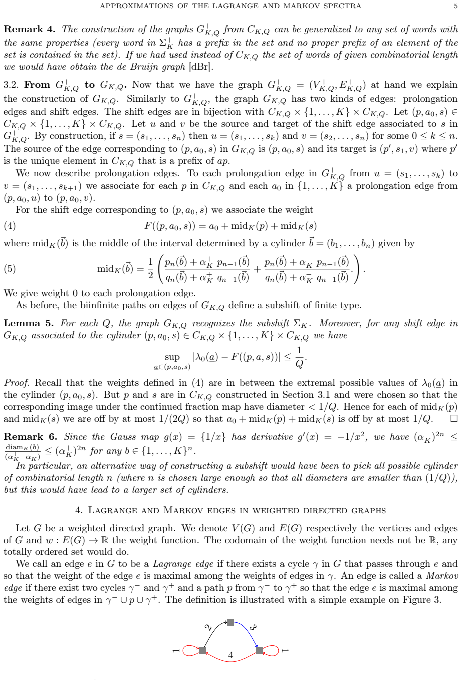
For $K\le4$, the load-bearing object is the weighted directed graph $G_{K,Q}$. Its vertices and edges encode the collection $C_{K,Q}$ of shortest cylinders of the Gauss map whose interval diameter is at most $1/Q$; a shift edge $(p,a_0,s)$ carries the weight $a_0+\mathrm{mid}_K(p)+\mathrm{mid}_K(s)$, the midpoint of the height function $\lambda_0$ over that cylinder, and the paper proves each such weight is within $1/Q$ of the true value of $\lambda_0$ on the cylinder. The spectral approximation is carried by Lagrange edges, meaning edges that are maximal on some directed cycle, and Markov edges, meaning edges maximal on a path running from one cycle into another. The graph size estimate $|G_{K,Q}|=\Theta(|C_{K,Q}|^2)=\Theta(Q^{2\mathrm{HD}(E_K)})$ follows from a diameter comparison, a lower bound on cylinder diameters, the uniform distortion bound for Gauss-map iterates, and a standard dimension-counting argument for cylinder covers; the total $O(Q^{3d_R})$ running time then comes from an $O(m^{3/2})$ step that extracts the spectral edge weights from a graph with $m$ edges.
What would settle it
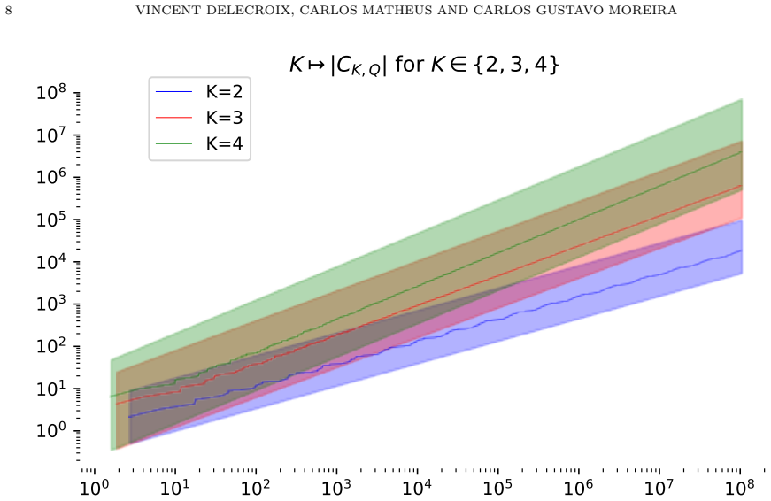
Take $K=2$ and count the cylinders $C_{2,Q}$ for $Q=10^2,10^3,\dots,10^8$; if $|C_{2,Q}|$ exceeds $4.98\cdot Q^{0.5313}$ at any of these sizes, the $\Theta(Q^{\mathrm{HD}(E_2)})$ bound behind the advertised running time is refuted. Independently, for a fixed $Q$, check the Hausdorff distance between the algorithm's output and $\mathcal{L}_2\cap[0,\sqrt{13}]$; any pair of points more than $1/Q$ apart would disprove the approximation claim.
Extended reading notes
Core claim
At the center of the paper is Theorem 1: for every $R>0$ there is an algorithm which, given $Q$, outputs finite sets that are $1/Q$-close in Hausdorff distance to both $\mathcal{L}\cap[0,R]$ and $\mathcal{M}\cap[0,R]$, and runs in time $O(Q^{3d_R})$. The exponents are explicit: $d_R<0.532$ when $R\le\sqrt{13}$, $d_R<0.706$ when $R\le2\sqrt{5}$, and $d_R<0.789$ when $R\le\sqrt{21}$, where $d_R$ is the Hausdorff dimension of the set $E_K$ of real numbers whose continued-fraction expansion uses only the digits $1,\dots,K$. The proof works by reducing the spectra to a finite combinatorial problem: the weights of Lagrange and Markov edges in a weighted directed graph $G_{K,Q}$ built from $(1/Q)$-cylinders of the Gauss map are shown to form a $1/Q$-Hausdorff approximation to the true spectra. The graph size is controlled by $|C_{K,Q}|=\Theta(Q^{\mathrm{HD}(E_K)})$, which follows from bounded distortion of Gauss-map iterates and the standard connection between cylinder counts and Hausdorff dimension.
Load-bearing premise
The advertised running time depends on two quoted numerical ingredients, rigorous bounds on the Hausdorff dimensions of the Cantor sets $E_2,E_3,E_4$ and a distortion bound of at most 4 for Gauss-map iterates, and if either of those failed the algorithm would still approximate correctly but could run slower than promised.
Editorial extensions
If this is right
- For each $R\le\sqrt{21}$, certified finite approximations of both spectra on $[0,R]$ exist at resolution $1/Q$ with running time polynomial in $Q$.
- Because the approximation is in Hausdorff distance, the output sets give both a lower and an upper bracket for every spectral point up to tolerance $1/Q$, so gaps and intervals in the spectra can be certified algorithmically.
- The exponent $d_R$ is a concrete, dimension-dependent number, so the same graph construction applies for any finite digit alphabet once the corresponding Cantor set dimension is known.
- The paper's implementation draws high-resolution pictures of $\mathcal{L}_2$ and $\mathcal{L}_3$ at precisions $1/150000$ and $1/3000$, showing the worst-case bounds are not merely asymptotic.
- The method also highlights why approximating the spectra by periodic orbits is far worse: the periodic-orbit route requires exponentially many periods, whereas the graph route stays polynomial.
Reading between the lines
- Inference: the same weighted-graph construction should transfer to any expanding one-dimensional map with bounded distortion and a digit-restricted alphabet, giving polynomial-time approximation of the associated spectra.
- Inference: since the approximation guarantee is uniform in $Q$ but the exponent comes from Hausdorff dimension, tighter rigorous dimension bounds for $E_2,E_3,E_4$ would directly improve the running time without changing the algorithm.
- Inference: the contrast with periodic-orbit approximation suggests that finite-type graph models, rather than periodic points, are the natural combinatorial skeleton for the fine structure of the Lagrange and Markov spectra.
- Inference: one could use this algorithm as a numerical probe for the local fractal structure of the spectra by measuring how the density of output points scales with $Q$ on small intervals, yielding empirical estimates of local Hausdorff dimension.
Signed reviews
Editorial analysis
A structured set of objections, weighed in public.
Referee Report
Summary. The paper presents an algorithm that, for any R>0 and any precision parameter Q, outputs finite sets that are 1/Q-close in Hausdorff distance to the intersections of the Lagrange and Markov spectra with [0,R]. The algorithm encodes the one-sided subshift with digits 1..K as a finite weighted graph whose edges are 1/Q-cylinders for the Gauss map, then computes the discrete analogues of Lagrange and Markov values on the graph. The number of graph edges is bounded by |C_{K,Q}|^2, and |C_{K,Q}| is shown to grow like Q^{HD(E_K)} using Hausdorff dimension estimates for continued fraction Cantor sets. The paper also gives a comparison with approximation by periodic orbits and includes high-resolution figures generated by an implementation whose code is publicly available.
Significance. If the main theorem is correct, this is the first polynomial-time procedure with explicit complexity bounds for Hausdorff approximation of both spectra, and it connects the algorithmic complexity to the Hausdorff dimension of the Cantor sets E_K. The paper has several concrete strengths: the central approximation step is derived from the definitions with explicit constants; the dimension estimates quoted from Jenkinson--Pollicott are rigorous and the constants in Theorem 13 are explicit; the implementation is publicly available; and the figures provide falsifiable outputs of the method. These strengths make the paper potentially valuable for computational number theory and dynamical systems, provided the correctness gaps identified below are addressed.
major comments (3)
- [Section 2 and Theorem 1] The range R≤√13 is incompatible with the choice K=2 at the endpoint. The maximum of L2 is L(2,1)=2√3≈3.464, while L(3)=√13≈3.606 belongs to L; the difference is about 0.141. Thus L∩[0,√13] is not contained in L2, so the graph G_{2,Q} cannot produce a 1/Q-close approximation for large Q. The same endpoint problem occurs at R=2√5 with K=3, since L(4)=2√5 belongs to L and is not in L3 if the claim about the minimum of L4\L3 is correct. The theorem should either state strict inequalities R<√13 and R<2√5, or the algorithm must explicitly adjoin the finitely many boundary values; the current wording is not correct.
- [Section 2] The assertion that 'the smallest and largest values of LK\L_{K-1} are respectively L(K) and L(1,K)' is load-bearing for Theorem 1 but is stated without proof or reference. Moreover, the immediately following bullets contain numerical errors: 'L(2,1)=√13 is the maximum of L2' should read 'L(2,1)=2√3', and 'L(4)=2√5 is the maximum of L4\L3' is inconsistent with Figure 1 unless 'minimum' is intended. Please provide a proof or a precise citation for the interval-containment property and correct these bullets.
- [Section 5, Theorem 9] The proof of Theorem 9 is written only for the Markov spectrum, with the Lagrange case dismissed as 'similar'. Since the Lagrange statement of Theorem 1 depends on this result, a complete argument is needed. In particular, the proof for the Lagrange case should show that a limsup value in LK can be approximated by an edge that is maximal on a cycle, taking into account that weights on the approximating cycle may exceed the target value only finitely often.
minor comments (4)
- [Abstract and title] The title/abstract contains a typo: 'APPROXIMA TIONS' should be 'APPROXIMATIONS'.
- [Section 3.2 and Lemma 10] The shift edges are described in Section 3.2 as being in bijection with CK,Q×{1,...,K}×CK,Q, but Lemma 10 counts them as |CK,Q|^2. The missing factor K does not change the order of magnitude, but the counting statement should be made consistent.
- [Remark 2] The statement that values R larger than √21 'do not make any sense' is too strong: L∩[0,R] is compact for every finite R and can be Hausdorff-approximated by finite sets. What the authors presumably mean is that the stated upper bounds on d_R do not apply, because one would need to include digits larger than 4.
- [Section 7, Proposition 15] In the Lagrange part of the proof, the text writes 'put t=L(a)∈L'; since a is restricted to ΣK, the statement is about LK, and the notation should reflect that.
Circularity Check
No significant circularity: the approximation guarantee follows directly from the cylinder construction, and the complexity exponents are supported by external, parameter-free results.
full rationale
The core approximation claim (Theorem 9) is self-contained: the graph G_{K,Q} is built from cylinders whose diameters are < 1/Q, the edge weights are cylinder midpoints, and Lemma 5 shows the midpoint weight is within 1/Q of every lambda_0 value in that cylinder. No Lagrange or Markov spectrum value is used as an input to fit a parameter, so the 1/Q closeness is not a renamed fit. The complexity part depends on Theorem 13, which is proved in the paper from a uniform distortion bound for iterates of the Gauss map and from standard Palis--Takens bounded-distortion estimates; the only numerical inputs are the rigorously computed Hausdorff-dimension bounds for E_2, E_3, E_4 due to Jenkinson and Pollicott, which are external to this paper. The citation to Moreira [Mor18] is a published, externally validated result used only for the distortion bound, not a self-citation that smuggles in the paper's own conclusion. The Section 2 assertion about the smallest and largest values of L_K \ L_{K-1}, and the evident typo confusing L(2,1) with L(3)=sqrt(13), are potential correctness concerns about whether the chosen alphabet K covers the required interval, but they are not circularity: the correctness proof of the approximation algorithm does not reduce to those assertions, and a failure there would affect the range of validity, not turn the derivation into a restatement of its inputs. The algorithm and its running-time analysis are therefore not circular; the result is a legitimate construction with independent complexity inputs.
Assumptions & free parameters
assumptions (5)
- standard math Perron's continued fraction formula for L(α) and the shift characterization of the Lagrange and Markov spectra.
- domain assumption The smallest and largest values of L_K\L_{K-1} are L(K) and L(1,K), respectively.
- domain assumption Rigorous interval bounds on the Hausdorff dimensions HD(E_2), HD(E_3), HD(E_4), namely 0.5312...0.5313, 0.7056...0.7057, and 0.7889...0.7890.
- domain assumption The distortion of iterates of the Gauss map on the relevant cylinders is bounded by 4.
- standard math Palis-Takens thermodynamic estimate: for a partition of E_K into cylinders C_{K,Q}, sums of derivative powers bracket 1.
Cite this review
Pith. "Pith review of Approximation of the Lagrange and Markov spectra." pith.science (2026). https://pith.science/paper/QIY6LQVH
@misc{pith2026190803773,
  author       = {Pith},
  title        = {Pith review of: Approximation of the Lagrange and Markov spectra},
  year         = {2026},
  howpublished = {\url{https://pith.science/paper/QIY6LQVH}},
  note         = {Machine review of arXiv:1908.03773}
}
read the original abstract
The (classical) Lagrange spectrum is a closed subset of the positive real numbers defined in terms of diophantine approximation. Its structure is quite involved. This article describes a polynomial time algorithm to approximate it in Hausdorff distance. It also extends to approximate the Markov spectrum related to infimum of binary quadratic forms.
Figures


Figures from the paper (2 more)

Reference graph
Works this paper leans on
- [1]
-
[2]
A. A. Berstein, The connections between the Markov and Lagrange spectra, Number-theoretic studies in the Markov spectrum and in the structural theory of set addition, pp. 16--49, 121--125. Kalinin. Gos. Univ., Moscow, 1973
work page 1973
-
[3]
T. Cusick and M. Flahive, The Markoff and Lagrange spectra, Mathematical Surveys and Monographs, 30. American Mathematical Society, Providence, RI, 1989. x+97 pp
work page 1989
-
[4]
R. Bradshaw, S. Behnel, D. S. Seljebotn, G. Ewing, et al., The Cython compiler, http://cython.org
-
[5]
N. G. deBruijn, A combinatorial problem, Nederl. Akad. Wetensch., Proc. 49 (1946), 758--764
work page 1946
-
[6]
G. A. Freiman, Noncoincidence of the Markoff and Lagrange spectra, Mat. Zametki 3 (1968), 195--200; English transl., Math. Notes 3 (1968),125--128
work page 1968
-
[7]
G. A. Freiman, The initial point of Hall's ray, Number-theoretic studies in the Markov spectrum and in the structural theory of set addition, pp. 87--120, 121--125. Kalinin. Gos. Univ., Moscow, 1973
work page 1973
-
[8]
B. Haeupler, T. Kavitha, R. Mathew, S. Sen, R. E. Tarjan, Faster algorithms for incremental topological ordering, in Proceedings of ICALP 2008. Springer
work page 2008
Show all 24 references
-
[9]
Kavitha, R
B Haeupler, T. Kavitha, R. Mathew, S. Sen, R. E. Tarjan, Incremental cycle detection, topological ordering, and strong component maintenance ACM Trans. Algorithms 8, No. 1, Paper No. 3, 33 p. (2012)
2012
-
[10]
Hensley, Continued fraction Cantor sets, Hausdorff dimension, and functional analysis, J
D. Hensley, Continued fraction Cantor sets, Hausdorff dimension, and functional analysis, J. Number Theory 40 (1992), no. 3, 336--358
1992
-
[11]
Hensley, A polynomial time algorithm for the Hausdorff dimension of continued fraction Cantor sets, J
D. Hensley, A polynomial time algorithm for the Hausdorff dimension of continued fraction Cantor sets, J. Number Theory 58 (1996), no. 1, 9--45
1996
-
[12]
J. D. Hunter Matplotlib: A 2D graphics environment, Computing in Science & Engineering, 9:3, p. 90--95 doi:10.1109/MCSE.2007.55 (2007)
2007 doi
-
[13]
Jenkinson, On the density of Hausdorff dimensions of bounded type continued fraction sets: the texan conjecture, Stochastics and Dynamics, vol 4, No 1 (2004) 63--76
O. Jenkinson, On the density of Hausdorff dimensions of bounded type continued fraction sets: the texan conjecture, Stochastics and Dynamics, vol 4, No 1 (2004) 63--76
2004
-
[14]
Jenkinson and M
O. Jenkinson and M. Pollicott, Computing the dimension of dynamically defined sets: E_2 and bounded continued fractions, Ergodic Theory Dynam. Systems 21 (2001), no. 5, 1429--1445
2001
-
[15]
Jenkinson and M
O. Jenkinson and M. Pollicott, Rigorous effective bounds on the Hausdorff dimension of continued fraction Cantor sets: a hundred decimal digits for the dimension of E_2 , Adv. Math. 325 (2018), 87--115
2018
-
[16]
Markov, Sur les formes quadratiques binaires ind\'efinies, Math
A. Markov, Sur les formes quadratiques binaires ind\'efinies, Math. Ann. 17 (1879), no. 3, 381--406
-
[17]
Markov, Sur les formes quadratiques binaires ind\'efinies II, Math
A. Markov, Sur les formes quadratiques binaires ind\'efinies II, Math. Ann. 17 (1880), no. 3, 379--399
-
[18]
Matheus and C
C. Matheus and C. G. Moreira, Fractal geometry of the complement of Lagrange spectrum in Markov spectrum, preprint 2018 available at arXiv:1803.01230, to appear in Comment. Math. Helv
2018 arXiv
-
[19]
C. G. Moreira, Geometric properties of the Markov and Lagrange spectra, Ann. of Math. 188 (2018), 145--170
2018
-
[20]
Morrison, A glimpse of the Markoff spectrum, preprint 2012 available at https://dca.ue.ucsc.edu/system/files/dca/2012/193/193.pdf
T. Morrison, A glimpse of the Markoff spectrum, preprint 2012 available at https://dca.ue.ucsc.edu/system/files/dca/2012/193/193.pdf
2012
-
[21]
Perron, \"Uber die approximation irrationaler Zahlen durch rationale II S.-B
O. Perron, \"Uber die approximation irrationaler Zahlen durch rationale II S.-B. Heidelberg Akad. Wiss. 8 (1921)
1921
-
[22]
Palis and F
J. Palis and F. Takens, Hyperbolicity and sensitive chaotic dynamics at homoclinic bifurcations, Fractal dimensions and infinitely many attractors. Cambridge Studies in Advanced Mathematics, 35. Cambridge University Press, Cambridge, 1993. x+234 pp. [1] ^ #1
1993
-
[23]
S ageMath, the S age M athematics S oftware S ystem ( V ersion 8.8) , The Sage Developers, 2019, https://www.sagemath.org
2019
-
[24]
Schecker, \"Uber die Menge der Zahlen, die als Minima quadratischer Formen auftreten, J
H. Schecker, \"Uber die Menge der Zahlen, die als Minima quadratischer Formen auftreten, J. Number Theory 9 (1977), no. 1, 121--141
1977
Reviewed August 14, 2026 · model on record in the stance chip above.
Discussion (0). Continue with ORCID to comment.