REVIEW 2 major objections 4 minor 58 references
Flats, spikes and crevices: the evolving shape of the inhomogeneous corner growth model
T0 review · 2 major / 4 minor · reviewed 2026-08-14 · deepseek-v4-flash
Pith's one-line read The paper proves explicit variational first-order asymptotics for the inhomogeneous exponential corner growth model and describes the limit shape with flats, spikes, and hidden crevices.
desk verdict A rigorous, explicit resolution of the Rains conjecture for inhomogeneous exponential LPP with a genuinely new description of spikes and crevices; the only real soft spot is a load-bearing but unproved permutation-invariance lemma imported from a cited paper. read the letter →
The pith
A machine-rendered reading of the paper's core claim, the machinery that carries it, and where it could break.
The reading
What carries the argument
The argument is carried by the increment-stationary last-passage processes $\tilde G^{a,b,z}$: couplings in which, for each $z$ in $(-\min a_m, \min b_n)$, the horizontal increments in a row are independent exponentials with rates $a_m(i)+z$ and the vertical increments in a column are independent exponentials with rates $b_n(j)-z$, so increments are stationary under translations (the Burke property). The mean of $\tilde G^{a,b,z}(m,n)$ is $M^{a,b,z}(m,n)$, and the true process is sandwiched around the unique minimizer $z$ of this convex function. Summable concentration bounds are obtained from exponential tail estimates for sums of independent exponentials and from controlling the probability that geodesics exit the rectangle through its boundary far from the origin. The only input from determinantal structure is the lemma, read off a cited distributional formula, that the law of $G^{a,b}(m,n)$ is invariant under permutations of the $a_m(i)$'s and $b_n(j)$'s; this invariance is what removes monotonicity assumptions from the left-tail bound.
What would settle it
For $m=n=2$, compute the exact distribution of $G^{a,b}(2,2)$ from the explicit formula cited in the paper for two choices of parameters, e.g. $(a_1,a_2)=(1,2)$, $(b_1,b_2)=(3,4)$, and for the permuted choices $(a_1,a_2)=(2,1)$, $(b_1,b_2)=(4,3)$. If the two distributions differ, the permutation-invariance lemma used to remove monotonicity in the left-tail bound is false, and the proof of Theorem 3.2 does not cover arbitrary rate parameters.
Extended reading notes
Core claim
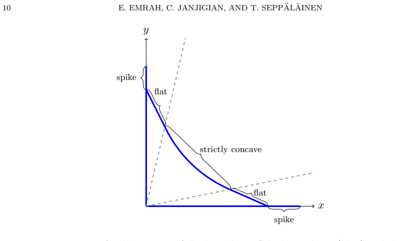
Let $G^{a,b}(m,n)$ be the largest total weight of an up-right path from $(1,1)$ to $(m,n)$ when the independent weights are exponential with rate $a_m(i)+b_n(j)$. The paper proves that, $P$-a.s., for all large $m+n$, $G^{a,b}(m,n)$ equals $M^{a,b}(m,n)=\inf_{z\in(-\min a_m, \min b_n)}\big(\sum_{i=1}^m (a_m(i)+z)^{-1} + \sum_{j=1}^n (b_n(j)-z)^{-1}\big)$ up to an error of smaller order than $m+n$, with explicit upper and lower tail bounds. When the empirical distributions of $a_m$ and $b_n$ converge vaguely to subprobability measures $\alpha$ and $\beta$ and the running minima converge to $a$ and $b$, the same result holds with the shape function $\gamma_{\alpha,\beta,a,b}(x,y)=\inf_{z\in(-a,b)}\big(x\int \alpha(da)/(a+z)+ y\int \beta(db)/(b-z)\big)$. The limit shape is then the sublevel set of this function together with explicit axis segments, and the paper describes exactly when its boundary is strictly concave, flat, or spiked. These results also prove the older variational conjecture formulated as Theorem 3.4 and imply explicit centerings for the disordered TASEP height and flux.
Load-bearing premise
The proof of the left-tail half of the main centering theorem relies on the unproved claim, quoted from a determinantal formula in the cited literature, that the law of $G^{a,b}(m,n)$ is unchanged when the row or column rate parameters are permuted; if that invariance failed, the centering theorem would only be established for monotone parameter sequences.
Editorial extensions
If this is right
- For any inhomogeneous exponential corner growth model satisfying the mild growth condition, leading-order growth values are computed by a one-dimensional convex minimization; the result does not require subadditive ergodic theory.
- When empirical rate distributions and running minima converge, the limit shape is completely explicit: the sublevel set of the shape function plus axis segments, with strictly concave boundary in one cone and flat boundary in the complementary regions.
- Axis spikes in the limit shape occur exactly when the supremum of the running minima exceeds its limit value, and flat segments adjacent to an axis occur exactly when a certain reciprocal-square integral is finite.
- Macroscopic spikes and crevices form along columns whose minimum rate is respectively above or below the limiting minimum; the limit shape encodes only the maximal spikes, not the crevices or smaller spikes.
- For TASEP with step initial condition and particle- and holewise disorder, the flux function and limiting particle profile are given by explicit formulas, so disorder effects on the current are computable.
Reading between the lines
- The same coupling-plus-variational strategy would likely transfer to other exactly solvable last-passage models that possess an analogous permutation-invariance property, even when full kernel asymptotics are unavailable.
- Because flat-segment formation is governed by the tail of $\alpha$ near its infimum, one can test for a geometric phase transition by tuning the decay of column parameters; the paper does not compute fluctuation orders across this transition.
- The fact that crevices vanish from the limit shape suggests that first-order shape functions miss a whole macroscopic structure; natural follow-up statistics are columnwise overshoot and undershoot magnitudes, and entropy of the height profile.
- Finite-size simulations against $t\mathcal{R}$ should reveal the predicted spike and crevice intervals; the paper gives such illustrations but not a quantitative goodness-of-fit criterion.
Signed reviews
Editorial analysis
A structured set of objections, weighed in public.
Referee Report
Summary. The paper studies the exactly solvable inhomogeneous corner growth model with exponential waiting times whose rates at site (i,j) are a_m(i)+b_n(j), with parameter collections varying in the rectangle size. The central result, Theorem 3.2, gives an almost sure first-order centering: G^{a,b}(m,n) equals the explicit variational quantity M^{a,b}(m,n) = inf_z [sum_i 1/(a_m(i)+z) + sum_j 1/(b_n(j)-z)] up to errors of order o(m+n). Under vague convergence of the empirical parameter distributions and convergence of running minima, Theorem 3.6 identifies the shape function as gamma_{alpha,beta,a,b}(x,y) = inf_z [x A_alpha(z) + y B_beta(z)]. Theorem 3.9 describes the limit shape, including flat segments, spikes, and the persistence of macroscopic spikes and crevices that are invisible in the limit shape. The paper also resolves a conjecture of Rains in this setting (Theorem 3.4) and derives limiting height, flux, and particle position formulas for disordered TASEP (Theorems 3.10 and 3.11). The method is based on concentration bounds, stationary-increment couplings, and boundary exit estimates for geodesics; the only integrable-probability input is the distributional invariance of the last-passage times under permutation of the parameters, stated as Lemma 4.4.
Significance. If the main theorems are fully established, this is a substantial contribution: it provides explicit, parameter-free variational formulas for the a.s. leading-order behavior of a non-stationary exactly solvable growth model, confirms a conjecture from Rains, and gives a detailed and partly surprising description of the limit shape, including flat segments and spikes alongside macroscopic features not visible in the limit. The concentration estimates and exit-probability arguments are worked out in detail, and the paper is careful to state the mild growth conditions under which the centering claims hold. The TASEP applications give useful explicit height and flux centerings in the presence of particlewise and holewise disorder. The main caveat is that one imported statement, Lemma 4.4, is load-bearing for all non-monotone parameter results and is not proved in the manuscript; this makes the current version conditional on the correctness and applicability of the cited determinantal formula.
major comments (2)
- [Section 4, Lemma 4.4] Lemma 4.4 is the only integrable-probability input in the paper and is used in a central way: in the proof of Lemma 4.7 the text states that 'by virtue of Lemma 4.4, the sequences (a_i) and (b_j) can be assumed to be nondecreasing without loss of generality', and Lemma 4.9 repeats this reduction. This monotone reduction is needed before the exit-probability bounds of Lemma 4.6 can be applied, and it ultimately supports the lower bound in Theorem 3.2, Corollary 3.3, Theorem 3.6, and Theorem 3.9. However, the proof of Lemma 4.4 is a single sentence citing equation (12) of [12], without verifying that the cited determinantal formula indeed applies to the two-index parameter collections in (1.7)-(1.8) and that it yields invariance under independent row and column permutations in the full generality needed here. This is a missing justification rather than an observed contradiction, but because the entire non-monotone regime depends on this assertion, the authors should either provide a self-contained proof of Lemma 4.4 or state the precise theorem from [12] with all hypotheses checked, including the regularity conditions on the parameters.
- [Section 5, proof of Theorem 3.2] The lower-bound part of Theorem 3.2 invokes Lemma 4.9, whose proof explicitly depends on Lemma 4.4 in the same way as Lemma 4.7 does. Thus the non-monotone case of the paper's central centering result is not independently established within the manuscript; it inherits the unresolved status of Lemma 4.4. If Lemma 4.4 is correct and applicable, the argument appears coherent, but as written the proof of the main theorem is incomplete for general parameter arrays satisfying only (1.8).
minor comments (4)
- [Abstract and Section 1.1] The abstract contains a typo: 'addivitely' should be 'additively'.
- [Section 1.5 and Section 3.9] Several corollaries and computations, including some parts of the flat-segment description and connections to earlier models, are deferred to the longer version [25]. The journal version should ensure that all claims stated as results are either proved in the text or accompanied by precise references to the longer version.
- [Section 3.6] The parametrization of the curved part of the limit shape is stated without a displayed derivation; adding the short computation that Phi(z) parametrizes the boundary would improve readability.
- [Section 4, Lemma 4.5] In the proof of Lemma 4.5, after the choice z = zeta - c(k-1)Delta/m, the constraint c < 1/3 is only introduced at the end; stating it before the estimate would make the argument easier to follow.
Circularity Check
No circularity: the central variational centering is an explicit function of the model rates and is proved by self-contained concentration arguments.
full rationale
The paper's main centering claim, Theorem 3.2, is that G^{a,b}(m,n) is almost surely within smaller order than m+n of M^{a,b}(m,n), where M^{a,b}(m,n) is defined in (3.3) as the explicit infimum over z of sums of reciprocal rates. This quantity is not fitted to the data or to the target limit; it is a deterministic function of the parameters, and the proof proceeds through right-tail bounds (Lemma 4.2), geodesic exit probabilities (Lemma 4.6), and left-tail bounds (Lemmas 4.7 and 4.9). The shape function in Theorem 3.6 is then obtained by a deterministic approximation of the centering under vague convergence of empirical rate measures (Lemma 7.2), not by assuming the desired limit. The only non-elementary probabilistic input, the permutation invariance in Lemma 4.4, is quoted from the external paper [12], not from the authors' own prior work, and it is used to reduce the left-tail estimate to the nondecreasing parameter case. The Burke-type stationarity of increments, stated in Section 2.3, is cited to [6] for constant parameters and to [22] for the extension; [22] is a published, independent prior result of one of the authors, and the stationarity property itself is a testable structural fact rather than the paper's conclusion. Several auxiliary claims are deferred to the longer version [25], such as an omitted complementary upper bound in Remark 3.9.1 and some corollaries in Section 3.9, but these deferrals concern supporting remarks and secondary examples, not the main derivation chain of the centering or limit shape. No equation is defined in terms of the quantity it is supposed to predict, and no fitted parameter is renamed as a prediction. The paper is therefore self-contained against external benchmarks for its central claims, and the residual concerns about cited or omitted proofs are matters of verification and completeness, not circularity.
Assumptions & free parameters
assumptions (4)
- domain assumption Waiting times are independent exponentials with rates a_i + b_j > 0 for all i,j (Section 1.4, Eq. (1.8)-(1.9)).
- standard math Permutation invariance of G^{a,b}(m,n) under row and column permutations (Lemma 4.4), cited from the determinantal formula in [12, Eq. (12)].
- domain assumption Vague convergence of empirical rate distributions and convergence of running minima, as in (3.16)-(3.17), for the shape function and limit shape theorems.
- standard math Standard tools from probability and analysis, including concentration inequalities for sums of independent exponentials (Lemma A.2), vague convergence criteria (Lemma A.4), and Cauchy transform estimates (Lemma A.5).
Cite this review
Pith. "Pith review of Flats, spikes and crevices: the evolving shape of the inhomogeneous corner growth model." pith.science (2026). https://pith.science/paper/QOLKTH33
@misc{pith2026190809319,
  author       = {Pith},
  title        = {Pith review of: Flats, spikes and crevices: the evolving shape of the inhomogeneous corner growth model},
  year         = {2026},
  howpublished = {\url{https://pith.science/paper/QOLKTH33}},
  note         = {Machine review of arXiv:1908.09319}
}
read the original abstract
We study the macroscopic evolution of the growing cluster in the exactly solvable corner growth model with independent exponentially distributed waiting times. The rates of the exponentials are given by an addivitely separable function of the site coordinates. When computing the growth process (last-passage times) at each site, the horizontal and vertical additive components of the rates are allowed to also vary respectively with the column and row number of that site. This setting includes several models of interest from the literature as special cases. Our main result provides simple explicit variational formulas for the a.s. first-order asymptotics of the growth process under a decay condition on the rates. Formulas of similar flavor were conjectured in arXiv:math/0004082, which we also establish. Subject to further mild conditions, we prove the existence of the limit shape and describe it explicitly. We observe that the boundary of the limit shape can develop flat segments adjacent to the axes and spikes along the axes. Furthermore, we record the formation of persistent macroscopic spikes and crevices in the cluster that are nonetheless not visible in the limit shape. As an application of the results for the growth process, we compute the flux function and limiting particle profile for the TASEP with the step initial condition and disorder in the jump rates of particles and holes. Our methodology is based on concentration bounds and estimating the boundary exit probabilities of the geodesics in the increment-stationary version of the model, with the only input from integrable probability being the distributional invariance of the last-passage times under permutations of columns and rows.
Figures


Figures from the paper (1 more)
Reference graph
Works this paper leans on
-
[12]
A. Borodin and S. P´ ech´ e. Airy kernel with two sets of parameters in directed percolation and random matrix theory. J. Stat. Phys. , 132(2):275–290, 2008
work page 2008
-
[1]
D. Ahlberg, M. Damron, and V. Sidoravicius. Inhomogeneous first-passage percolation. Electron. J. Probab., 21:Paper No. 4, 19, 2016
work page 2016
-
[2]
A. Auffinger and M. Damron. Differentiability at the edge of the percolation cone and related results in first-passage percolation. Probab. Theory Related Fields, 156(1-2):193–227, 2013
work page 2013
-
[3]
A. Auffinger, M. Damron, and J. Hanson. 50 years of first-passage percolation , volume 68 of University Lecture Series. American Mathematical Society, Providence, RI, 2017
work page 2017
-
[4]
C. Bahadoran and T. Bodineau. Quantitative estimates for the flux of TASEP with dilute site disorder. Electron. J. Probab., 23:Paper No. 44, 44, 2018
work page 2018
-
[5]
J. Baik, G. Ben Arous, and S. P´ ech´ e. Phase transition of the largest eigenvalue for nonnull complex sample covariance matrices. Ann. Probab., 33(5):1643–1697, 2005
work page 2005
-
[6]
M. Bal´ azs, E. Cator, and T. Sepp¨ al¨ ainen. Cube root fluctuations for the corner growth model associated to the exclusion process. Electron. J. Probab., 11:no. 42, 1094–1132 (electronic), 2006
work page 2006
-
[7]
G. Barraquand. A phase transition for q-TASEP with a few slower particles. Stochastic Process. Appl., 125(7):2674–2699, 2015
work page 2015
Show all 58 references
-
[8]
R. Basu, V. Sidoravicius, and A. Sly. Last-passage percolation with a defect line and the solution of the slow bond problem. arXiv:1408.3464, 2016
2016 arXiv
-
[9]
Beffara, V
V. Beffara, V. Sidoravicius, and M. Eulalia Vares. Randomized polynuclear growth with a columnar defect. Probab. Theory Related Fields, 147(3-4):565–581, 2010
2010
-
[10]
Ben Arous and I
G. Ben Arous and I. Corwin. Current fluctuations for TASEP: a proof of the Pr¨ ahofer-Spohn conjecture. Ann. Probab., 39(1):104–138, 2011
2011
-
[11]
Benjamini, P
I. Benjamini, P. A. Ferrari, and C. Landim. Asymmetric conservative processes with random rates. Sto- chastic Process. Appl., 61(2):181–204, 1996
1996
-
[13]
J. Calder. Directed last passage percolation with discontinuous weights. J. Stat. Phys. , 158(4):903–949, 2015
2015
-
[14]
H. Cohn, N. Elkies, and J. Propp. Local statistics for random domino tilings of the Aztec diamond. Duke Math. J., 85(1):117–166, 1996
1996
-
[15]
Corwin, Z
I. Corwin, Z. Liu, and D. Wang. Fluctuations of TASEP and LPP with general initial data. Ann. Appl. Probab., 26(4):2030–2082, 2016
2016
-
[16]
M. Damron. Random growth models: shape and convergence rate. In Random growth models, volume 75 of Proc. Sympos. Appl. Math. , pages 1–37. Amer. Math. Soc., Providence, RI, 2018
2018
-
[17]
Damron, F
M. Damron, F. Rassoul-Agha, and T. Sepp¨ al¨ ainen. Random growth models.Notices Amer. Math. Soc. , 63(9):1004–1008, 2016. CORNER GROWTH MODEL 45
2016
-
[18]
A. B. Dieker and J. Warren. On the largest-eigenvalue process for generalized Wishart random matrices. ALEA Lat. Am. J. Probab. Math. Stat. , 6:369–376, 2009
2009
-
[19]
R. Durrett. Probability: theory and examples . Cambridge Series in Statistical and Probabilistic Mathe- matics. Cambridge University Press, Cambridge, fourth edition, 2010
2010
-
[20]
Durrett and T
R. Durrett and T. M. Liggett. The shape of the limit set in Richardson’s growth model. Ann. Probab., 9(2):186–193, 1981
1981
-
[21]
M. Eden. A two-dimensional growth process. In Proc. 4th Berkeley Sympos. Math. Statist. and Prob., Vol. IV, pages 223–239. Univ. California Press, Berkeley, Calif., 1961
1961
-
[22]
E. Emrah. Limit shapes for inhomogeneous corner growth models with exponential and geometric weights. Electron. Commun. Probab., 21:Paper No. 42, 16, 2016
2016
-
[23]
Emrah and C
E. Emrah and C. Janjigian. Large deviations for some corner growth models with inhomogeneity. Markov Process. Related Fields, 23(2):267–312, 2017
2017
-
[24]
Emrah, C
E. Emrah, C. Janjigian, and T. Sepp¨ al¨ ainen. Busemann functions and geodesics in solvable inhomogeneous exponential last passage percolation. In preparation
-
[25]
Emrah, C
E. Emrah, C. Janjigian, and T. Sepp¨ al¨ ainen. Flats, spikes and crevices: the evolving shape of the inho- mogeneous corner growth model. arXiv:1908.09319v1
1908 arXiv
-
[26]
G. B. Folland. Real analysis: Modern techniques and their applications . Pure and Applied Mathematics. John Wiley & Sons Inc., New York, second edition, 1999
1999
-
[27]
Georgiou and F
N. Georgiou and F. Ciech. Last-passage percolation in an exponential environment with discontinuous rates. arXiv:1808.00917, 2018
2018 arXiv
-
[28]
Georgiou, F
N. Georgiou, F. Rassoul-Agha, and T. Sepp¨ al¨ ainen. Variational formulas and cocycle solutions for directed polymer and percolation models. Comm. Math. Phys. , 346(2):741–779, 2016
2016
-
[29]
Gravner, C
J. Gravner, C. A. Tracy, and H. Widom. Fluctuations in the composite regime of a disordered growth model. Comm. Math. Phys. , 229(3):433–458, 2002
2002
-
[30]
Gravner, C
J. Gravner, C. A. Tracy, and H. Widom. A growth model in a random environment. Ann. Probab., 30(3):1340–1368, 2002
2002
-
[31]
Halpin-Healy and Y
T. Halpin-Healy and Y. Zhang. Kinetic roughening phenomena, stochastic growth, directed polymers and all that. Aspects of multidisciplinary statistical mechanics. Physics Reports, 254:215–414, 1995
1995
-
[32]
S. A. Janowsky and J. L. Lebowitz. Finite-size effects and shock fluctuations in the asymmetric simple- exclusion process. Phys. Rev. A , 45:618–625, 1992
1992
-
[33]
S. A. Janowsky and J. L. Lebowitz. Exact results for the asymmetric simple exclusion process with a blockage. J. Statist. Phys. , 77(1-2):35–51, 1994
1994
-
[34]
Jockusch, J
W. Jockusch, J. Propp, and P. Shor. Random domino tilings and the arctic circle theorem. arXiv:math/9801068
-
[35]
Johansson
K. Johansson. Random growth and random matrices. In European Congress of Mathematics, Vol. I (Barcelona, 2000), volume 201 of Progr. Math., pages 445–456. Birkh¨ auser, Basel, 2001
2000
-
[36]
Johansson
K. Johansson. On some special directed last-passage percolation models. In Integrable systems and random matrices, volume 458 of Contemp. Math., pages 333–346. Amer. Math. Soc., Providence, RI, 2008
2008
-
[37]
Kandel and D
D. Kandel and D. Mukamel. Defects, interface profile and phase transitions in growth models. Europhysics Letters, 20(4):325–229, 1992
1992
-
[38]
Knizel, L
A. Knizel, L. Petrov, and A. Saenz. Generalizations of TASEP in discrete and continuous inhomogeneous space. Comm. Math. Phys. , 372(3):797–864, 2019
2019
-
[39]
Krug and P
J. Krug and P. Ferrari. Phase transitions in driven diffusive systems with random rates. J. Phys. A , 29:L465–L471, 1996
1996
-
[40]
Krug and H
J. Krug and H. Spohn. Kinetic roughening of growing surfaces. In C. Godr` eche, editor, Solids far from equilibrium, Collection Al´ ea-Saclay: Monographs and Texts in Statistical Physics, 1, pages 117–130. Cambridge University Press, Cambridge, 1992
1992
-
[41]
Marchand
R. Marchand. Strict inequalities for the time constant in first passage percolation. Ann. Appl. Probab. , 12(3):1001–1038, 2002
2002
-
[42]
J. B. Martin. Limiting shape for directed percolation models. Ann. Probab., 32(4):2908–2937, 2004
2004
-
[43]
J. B. Martin. Last-passage percolation with general weight distribution. Markov Process. Related Fields, 12(2):273–299, 2006
2006
-
[44]
J. R. Munkres. Topology. Prentice-Hall, Inc., Upper Saddle River, N.J., second edition, 2000
2000
-
[45]
Okounkov
A. Okounkov. Infinite wedge and random partitions. Selecta Math. (N.S.) , 7(1):57–81, 2001
2001
-
[46]
E. Rains. A mean identity for longest increasing subsequence problems. arXiv:math/0004082, 2000. 46 E. EMRAH, C. JANJIGIAN, AND T. SEPP ¨AL¨AINEN
2000 arXiv
-
[47]
Richardson
D. Richardson. Random growth in a tessellation. Proc. Cambridge Philos. Soc. , 74:515–528, 1973
1973
-
[48]
H. Rost. Nonequilibrium behaviour of a many particle process: density profile and local equilibria. Z. Wahrsch. Verw. Gebiete, 58(1):41–53, 1981
1981
-
[49]
W. Rudin. Principles of mathematical analysis . McGraw-Hill Book Co., New York-Auckland-D¨ usseldorf, third edition, 1976. International Series in Pure and Applied Mathematics
1976
-
[50]
Sch¨ utz and E
G. Sch¨ utz and E. Domany. Phase transitions in an exactly soluble one-dimensional exclusion process. J. Statist. Phys., 72(1-2):277–296, 1993
1993
-
[51]
Sepp¨ al¨ ainen
T. Sepp¨ al¨ ainen. Hydrodynamic scaling, convex duality and asymptotic shapes of growth models.Markov Process. Related Fields, 4(1):1–26, 1998
1998
-
[52]
Sepp¨ al¨ ainen
T. Sepp¨ al¨ ainen. Lecture notes on the corner growth model. http://www.math.wisc.edu/~seppalai/ cornergrowth-book/ajo.pdf, 2009
2009
-
[53]
Sepp¨ al¨ ainen
T. Sepp¨ al¨ ainen. The corner growth model with exponential weights. InRandom growth models, volume 75 of Proc. Sympos. Appl. Math., pages 133–201. Amer. Math. Soc., Providence, RI, 2018.arXiv:1709.05771
2018 arXiv
-
[54]
Sepp¨ al¨ ainen and J
T. Sepp¨ al¨ ainen and J. Krug. Hydrodynamics and platoon formation for a totally asymmetric exclusion model with particlewise disorder. J. Statist. Phys. , 95(3-4):525–567, 1999
1999
-
[55]
A. Sly. Note on the flux for TASEP with general disorder. arXiv:1609.06589, 2016
2016 arXiv
-
[56]
F. Spitzer. Interaction of Markov processes. Advances in Math., 5:246–290 (1970), 1970
1970
-
[57]
Tripathy and M
G. Tripathy and M. Barma. Driven lattice gases with quenched disorder: Exact results and different macroscopic regimes. Phys. Rev. E , 58(2):1911–1926, 1998
1911
-
[58]
D. E. Wolf and L. Tang. Inhomogeneous growth processes. Physical Review Letters , 65(13):1591–1594, 1990. Elnur Emrah, KTH Royal Institute of Technology, Department of Mathematics, SE-100 44 Stockholm, Sweden. Email address: elnur@kth.se URL: https://sites.google.com/view/elnu...
1990
Reviewed August 14, 2026 · model on record in the stance chip above.
Discussion (0). Continue with ORCID to comment.