REVIEW 5 major objections 6 minor 119 references
Transformers Beyond Order: A Chaos-Markov-Gaussian Framework for Short-Term Sentiment Forecasting of Any Financial OHLC timeseries Data
T0 review · 5 major / 6 minor · reviewed 2026-08-07 · deepseek-v4-flash
Pith's one-line read A hybrid Chaos-Markov-Gaussian framework is claimed to forecast next-day opening sentiment across 160 market indices with 76.7% accuracy, beating LSTM and other baselines under identical training conditions.
desk verdict The accuracy claim is unevaluable as written: no mapping from the six-class target to the binary daybreak metric, and the 'any' rule can score both directions correct on the same day. read the letter →
The pith
A machine-rendered reading of the paper's core claim, the machinery that carries it, and where it could break.
The reading
What carries the argument
The central object is the CMG pipeline: a MACD-intersection-derived target variable verified as chaotic, a transformer encoder-decoder whose cross-attention uses a transposed causal mask, a six-class Gaussian binning scheme for sentiment strength, and a final LSTM layer. The transposed mask flips ordinary causal masking so the model attends only to current and future tokens and never to past tokens; the paper presents this as the mechanism that enforces the Markov property. The LSTM layer is included to restore sequential memory that the transformer lacks, and the Gaussian binning maps continuous sentiment strength onto a standard normal distribution. What this machinery is doing is connecting three mathematical formalisms to a single deep-learning architecture, then claiming that the connection improves forecasting accuracy.
What would settle it
Re-run the 160-index evaluation with the transposed cross-attention mask replaced by the standard causal mask while keeping all other settings identical; if the standard-mask model reaches or exceeds 0.7672 accuracy, the Markov-enforcing mask is not the source of CMG's reported advantage.
Extended reading notes
Core claim
The paper's central claim is that its Chaos-Markov-Gaussian (CMG) framework forecasts short-term market sentiment more accurately than existing baselines under the same training conditions. Daybreak sentiment is scored correct when the next day's opening quarter contains a price on the predicted side of the previous close. On 160 indices from more than 16 markets, CMG's average accuracy is 0.7672 versus 0.7605 for LSTM, 0.7602 for BiLSTM, and lower for GRU and the statistical and machine-learning models. The paper reports paired t-tests and Wilcoxon signed-rank tests with p-values below 0.05 against every baseline and interprets this as evidence that the gain is real rather than random. It further claims the framework is resource-efficient, using one dedicated transformer per index and a smaller model file than the BiLSTM baseline.
Load-bearing premise
The accuracy claim rests on the premise that a model forbidden from attending to any past tokens can still forecast next-day sentiment from a single current state, and the paper does not test that mask against a standard causal mask.
Editorial extensions
If this is right
- If the claim holds, daybreak sentiment for the first quarter of the next trading day is predictable at roughly 76.7 percent average accuracy across a wide range of global indices without instrument-specific tuning.
- The one-model-per-index design implies the framework can run in resource-constrained or edge settings, since it avoids training a single giant global model and uses less storage than the BiLSTM baseline.
- The significant paired-test results imply the small accuracy margin over LSTM is unlikely to be chance, so even standardized, no-feature-engineering evaluations can separate model performance.
- The demonstrated chaos metrics (positive Lyapunov exponents, low-dimensional correlation dimensions) imply the target series carry exploitable nonlinear structure rather than pure noise.
Reading between the lines
- The paper does not report an ablation swapping the transposed mask for the standard causal mask, so a direct comparison would show whether the Markov mechanism is responsible for the accuracy gain or is merely a constraint the model overcomes.
- The paper's own framing implies that recent OHLC history drives daybreak sentiment, which is in tension with a mask that forbids all past tokens; a test that feeds the previous day's close explicitly would resolve whether the Markov assumption helps or hurts.
- Because the reported accuracy gap over LSTM is 0.0067, the practical trading value of CMG would hinge on replication and on whether this edge persists after transaction costs and on out-of-sample periods.
- The chaos component is verified on the constructed target, not on the model's internal dynamics, so the framework's contribution would be clearer if experiments removed the chaotic target transformation and measured accuracy directly.
Editorial analysis
A structured set of objections, weighed in public.
Referee Report
Summary. The paper introduces a Chaos-Markov-Gaussian (CMG) framework for short-term sentiment forecasting of financial OHLC time series. The target variable is constructed from price changes between consecutive MACD/signal-line crossings, mapped to six discrete classes using Gaussian percentiles, and modeled by a transformer with a transposed causal mask plus an LSTM layer. The authors evaluate the framework on 160 market indices by comparing its average daybreak sentiment accuracy (0.7672) with statistical, machine learning, and deep learning baselines (best baseline LSTM: 0.7605), reporting statistically significant paired t-test and Wilcoxon signed-rank test p-values. The paper also provides chaos diagnostics for the constructed target variable and a public code repository.
Significance. If the reported comparison were valid, the CMG framework would offer a resource-efficient and broadly applicable short-term sentiment forecaster. The paper has notable strengths: a large multi-market dataset (160 indices), a diverse set of baselines, paired statistical tests, reproducibility through a public code repository, and explicit chaos diagnostics. However, the central claim rests on an evaluation protocol that is not connected to the training objective, and the reported accuracy differences are so small that the metric definition determines the outcome. As presented, the evidence does not establish that the CMG framework outperforms the baselines for the stated daybreak sentiment task.
major comments (5)
- [§4.1.3 and §1] The training target and the evaluation metric are mismatched. The target is y_t = P_t' - P_t, a price change between two successive MACD/signal-line intersections, whose horizon is the time until the next crossing; this is binned into six classes {-3,-2,-1,1,2,3} (§3.4.1). The evaluation metric is binary daybreak sentiment: whether the previous close is above or below 'any price within the first quarter of the next trading day' (§1). No mapping from the six MACD-crossing classes to these binary labels is specified, and there is no neutral class, so it is undefined how the trained model's output is converted into a bullish/bearish prediction. Consequently, Table 2 does not measure what it claims to measure, and the p-values in Tables 3-4 are uninterpretable as evidence about daybreak sentiment accuracy.
- [§1 (sentiment accuracy metric)] The daybreak sentiment metric is not a well-defined scoring rule. The text says a bullish prediction is correct if the previous close is 'less than any price within the first quarter' and bearish if it is 'greater than any price'; with the natural existential reading of 'any', whenever the previous close lies strictly between the first-quarter high and low—a common configuration in daily OHLC data—both a bullish and a bearish prediction are scored as correct. The phrase 'All other cases are considered incorrect' does not resolve this ambiguity. Because all models receive the same free credit on such days, the reported average accuracy differences (e.g., CMG 0.7672 vs. LSTM 0.7605) are compressed and cannot support the statistical conclusions. The authors must define a mutually exclusive and exhaustive labeling rule (e.g., compare the close with the first-quarter midpoint, or use 'above all'/'below all') and report the fraction of days affected by the ambiguity.
- [§3.3.1 and §3.5.3] The transposed causal mask is inconsistent with the paper's own task description. Section 1 states that short-term sentiment forecasting 'relies heavily on recent OHLC data,' but §3.3.1 defines a mask that lets the model 'attend only to the current and future tokens, and explicitly preventing access to past tokens,' and the preprocessing 'retains only the current state.' If each input instance contains only the current state, the model cannot see the previous day's close, trend, or any other recent features that the paper says drive daybreak sentiment. No ablation or analysis is reported showing that this mask improves accuracy, so the claimed alignment with the Markov property is asserted rather than demonstrated. The authors need to clarify what tokens are actually in the input sequence and provide an ablation of the masking choice.
- [§4.1.3 and §4.1.4] The chaos component is circular as presented. The target variable is constructed from MACD crossings, then tested for chaotic behavior (§4.1.4), and the positive test results are used to justify the chaos-based architecture of the CMG model. This does not validate the forecasting value of the chaos framing; it only shows that the constructed target has certain statistical properties. The self-referential note in §3.2 that references [41]–[46] 'are drawn from external literature where mildly similar methodologies or theoretical inspirations have been applied' further indicates that the chaos component is not independently grounded. The authors should either provide a non-circular justification for why the chaos transformation improves prediction or remove the chaos framing from the load-bearing claims.
- [§4.1.2 and §4.2.1] The claim of 'no feature engineering' in the abstract and §1 is contradicted by the methodology. Section 4.1.2 describes an extensive suite of technical indicators (SMA, EMA, MACD, RSI, Bollinger Bands, and many more), and Appendix B lists hundreds of engineered columns. All models are trained on these features, so the comparison is not feature-engineering-free. In addition, the resource-efficiency claim is unsupported: Table 5 reports only model file sizes, with no training time, inference time, or computational cost measurements. The authors should state exactly what 'no feature engineering' means and provide direct efficiency measurements for the claims of speed and resource reduction.
minor comments (6)
- [§1] The phrase 'first quarter of the next trading day' is ambiguous: it could mean the first 25% of trading hours, the first quarter-hour, or another interval. This needs a precise time definition because the evaluation metric depends on it.
- [§3.4.1] The 'Gaussian Process component' is not a Gaussian process in the usual sense: the method only discretizes the target variable using percentiles of a standard normal distribution. No GP prior, kernel, or posterior inference is used. Please rename this component or describe the actual Gaussian modeling step.
- [§4.1.5] The standardization strategy is described only verbally: per-day z-scoring for features and global cumulative standardization for targets. The exact formulas and the handling of the first day (when no previous data exists) should be stated explicitly for reproducibility.
- [References] There are several reference formatting errors; for example, reference [1] combines two separate works into one entry, and some entries are incomplete. The list should be checked against a standard citation format.
- [Table 1] The column header 'DF A α' should be 'DFA α', and some index tickers in Appendix A (e.g., 'BSE.PR.OWER') appear to be misspelled or truncated; please verify the ticker list.
- [§5] The statistical analysis would benefit from effect sizes and confidence intervals for the accuracy differences, in addition to p-values, and from a multiple-comparison correction given that eight pairwise tests are reported.
Circularity Check
The Gaussian and chaos pillars are self-definitional: the six-class target is Gaussian by binning, and the chaos tests validate a target built to mimic chaos; the headline accuracy claim is additionally not a well-defined function of the model outputs.
-
self definitional
[Section 3.4.1, 'Probabilistic Forecasting with GPs']
"The continuous output is discretized into six sentiment classes, mapped onto a standard normal distribution. These classes correspond to the intervals defined by the 50th, 75th, and 100th percentiles on both sides of the distribution, with class labels assigned as: -3, -2, -1, 1, 2, and 3. This binning strategy enables the model to capture graded sentiment intensity while preserving the probabilistic structure of the Gaussian distribution."
The Gaussian property is imposed by the construction itself: the target is binned at quantiles of a standard normal, so the resulting six classes are Gaussian by definition. The paper then invokes this binning as the 'Gaussian process' component and claims it provides probabilistic forecasts and confidence bounds. No Gaussian process is fitted or tested; the probabilistic claim is an artifact of the chosen binning rather than an independent constraint on the data or a derived result.
-
self definitional
[Section 3.2 (embedding chaos) and Section 4.1.4 (Verification of Chaotic Behavior)]
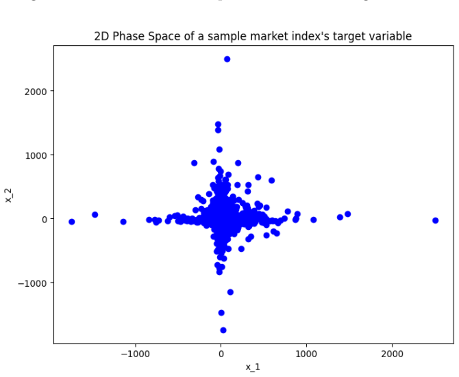
"Chaos theory is not only used to analyse the data but is actively embedded into the forecasting task by transforming the target variable to mimic the characteristics of chaotic systems... Passing these tests confirms that the target variable exhibits chaotic properties suitable for modelling with the CMG framework."
The target variable is deliberately engineered to mimic chaotic systems, and the same engineered variable is then tested with Lyapunov exponents, correlation dimension, and entropy measures. A positive result is presented as confirmation that short-term sentiment follows a chaotic process, but it only confirms the construction. This self-referential validation is then used to justify the chaos-based architecture, so the justification reduces to an input assumption renamed as an empirical finding.
full rationale
The most defensible reading is partial circularity. The framework's two mathematical pillars are validated by construction: the Gaussian component is only a normal-quantile binning of the engineered target, and the chaos component is confirmed by running chaos tests on a target that was itself built to mimic chaotic behavior. These steps do not provide independent support for the claimed chaos/Gaussian modeling. Separately, and not a circularity per se, the central accuracy comparison is difficult to interpret: the model is trained on six-class MACD-intersection targets (Section 4.1.3) while Table 2 reports 'daybreak sentiment accuracy' defined by the next day's first-quarter OHLC, with no explicit mapping from the six classes to the binary bullish/bearish rule; the p-values in Tables 3-4 therefore inherit the ambiguity of the accuracy measure. I did not find self-citation or ansatz-smuggling issues; the cited external literature is not load-bearing in a circular way. Overall score reflects that two supporting 'results' reduce by construction, although the headline comparison still has independent (if uninterpreted) empirical content.
Assumptions & free parameters
free parameters (4)
- MACD parameters (12, 26, 9) =
12, 26, 9
- Six sentiment class percentile boundaries =
50th, 75th, 100th percentiles on each side of the standard normal
- Technical indicator windows and parameters =
e.g., ATR 5 15, RSI 14, BB 5 2.0
- Single transformer layer, hidden size, heads, LSTM cells =
unspecified
assumptions (4)
- domain assumption The target series derived from MACD crossing price differences is a meaningful representation of short-term sentiment.
- domain assumption The constructed target variable is chaotic, and this justifies the chaos-based model design.
- ad hoc to paper The transposed causal mask enforces the Markov property and improves forecasting.
- ad hoc to paper The six discrete Gaussian-derived classes can be trained as a proxy for the binary daybreak sentiment evaluation.
Cite this review
Pith. "Pith review of Transformers Beyond Order: A Chaos-Markov-Gaussian Framework for Short-Term Sentiment Forecasting of Any Financial OHLC timeseries Data." pith.science (2026). https://pith.science/paper/QP3AEZSS
@misc{pith2026250617244,
  author       = {Pith},
  title        = {Pith review of: Transformers Beyond Order: A Chaos-Markov-Gaussian Framework for Short-Term Sentiment Forecasting of Any Financial OHLC timeseries Data},
  year         = {2026},
  howpublished = {\url{https://pith.science/paper/QP3AEZSS}},
  note         = {Machine review of arXiv:2506.17244}
}
read the original abstract
Short-term sentiment forecasting in financial markets (e.g., stocks, indices) is challenging due to volatility, non-linearity, and noise in OHLC (Open, High, Low, Close) data. This paper introduces a novel CMG (Chaos-Markov-Gaussian) framework that integrates chaos theory, Markov property, and Gaussian processes to improve prediction accuracy. Chaos theory captures nonlinear dynamics; the Markov chain models regime shifts; Gaussian processes add probabilistic reasoning. We enhance the framework with transformer-based deep learning models to capture temporal patterns efficiently. The CMG Framework is designed for fast, resource-efficient, and accurate forecasting of any financial instrument's OHLC time series. Unlike traditional models that require heavy infrastructure and instrument-specific tuning, CMG reduces overhead and generalizes well. We evaluate the framework on market indices, forecasting sentiment for the next trading day's first quarter. A comparative study against statistical, ML, and DL baselines trained on the same dataset with no feature engineering shows CMG consistently outperforms in accuracy and efficiency, making it valuable for analysts and financial institutions.
Figures


Figures from the paper (2 more)


Reference graph
Works this paper leans on
-
[41]
Pathak, J., Lu, Z., Hunt, B. R., Girvan, M., & Ott, E. (2018). Model-free prediction of large spatiotemporally chaotic systems from data: A reservoir computing approach. Physical Review Letters, 120(2), 024102
work page 2018
-
[46]
Chen, S. H., & Yeh, C. H. (2001). Evolving traders and the business school with genetic pro- gramming: A new architecture of the agent-based artificial stock market. Journal of Economic Dynamics and Control, 25(3-4), 363–393
work page 2001
-
[1]
Box, G. E. P., Jenkins, G. M., & Reinsel, G. C. (2008). Time Series Analysis: Forecasting and Control (4th ed.). Wiley.Bollerslev, T. (1986). Generalized Autoregressive Conditional Het- eroskedasticity.Journal of Econometrics, 31(3), 307–327. 21
2008
-
[2]
Li, W., Liu, J., & Le, J. (2005). Using GARCH-GRNN model to forecast financial time series. In A. Yazici & C. Sener (Eds.), Computer and Information Sciences - ISCIS 2005 (Lecture Notes in Computer Science, Vol. 3733, pp. 499–507). Springer
2005
-
[3]
Engle, R. F. (1982). Autoregressive Conditional Heteroskedasticity with Estimates of the Vari- ance of United Kingdom Inflation. Econometrica, 50(4), 987–1007
1982
-
[4]
Zhang, G. P. (2003). Time series forecasting using a hybrid ARIMA and neural network model. Neurocomputing, 50, 159–175
2003
-
[5]
Tetlock, P. C. (2007). Giving content to investor sentiment: The role of media in the stock market. The Journal of Finance, 62(3), 1139–1168
2007
-
[6]
Norris, J. R. (1998). Markov Chains. Cambridge University Press
1998
Show all 119 references
-
[7]
Hamilton, J. D. (1989). A new approach to the economic analysis of nonstationary time series and the business cycle. Econometrica, 57(2), 357–384
1989
-
[8]
Kritzman, M., Li, Y., Page, S., & Rigobon, R. (2012). Principal Components as a Measure of Systemic Risk. The Journal of Portfolio Management, 38(4), 112–126
2012
-
[9]
Rabiner, L. R. (1989). A tutorial on hidden Markov models and selected applications in speech recognition. Proceedings of the IEEE, 77(2), 257–286
1989
-
[10]
Gleick, J. (1987). Chaos: Making a New Science. Viking
1987
-
[11]
Peters, E. E. (1991). Chaos and Order in the Capital Markets: A New View of Cycles, Prices, and Market Volatility. John Wiley & Sons
1991
-
[12]
Mandelbrot, B. B. (1982). The Fractal Geometry of Nature. W. H. Freeman
1982
-
[13]
A., & LeBaron, B
Scheinkman, J. A., & LeBaron, B. (1989). Nonlinear dynamics and stock returns. Journal of Business, 62(3), 311–337
1989
-
[14]
Hsieh, D. A. (1991). Chaos and nonlinear dynamics: Application to financial markets. The Journal of Finance, 46(5), 1839–1877
1991
-
[15]
H., & Shaw, C
Abraham, R. H., & Shaw, C. D. (1992). Dynamics: The Geometry of Behavior. Addison- Wesley
1992
-
[16]
E., & Williams, C
Rasmussen, C. E., & Williams, C. K. I. (2006). Gaussian Processes for Machine Learning. MIT Press
2006
-
[17]
B., Polson, N
Heaton, J. B., Polson, N. G., & Witte, J. H. (2017). Deep learning in finance. Annual Review of Financial Economics, 9, 145–181
2017
-
[18]
Lam, P., & Mirza, H. (2015). Gaussian Process for financial sentiment prediction. Proceedings of the International Conference on Machine Learning Applications
2015
-
[19]
S., Shen, X., & Cai, J
Liu, H., Ong, Y. S., Shen, X., & Cai, J. (2018). When Gaussian process meets big data: A review of scalable GPs. IEEE Transactions on Neural Networks and Learning Systems, 31(11), 4405–4423. 22
2018
-
[20]
Wang, Z., Hutter, F., Zoghi, M., Matheson, D., & De Freitas, N. (2013). Bayesian optimiza- tion in high dimensions via random embeddings. Proceedings of the 23rd International Joint Conference on Artificial Intelligence
2013
-
[21]
Fischer, T., & Krauss, C. (2018). Deep learning with long short-term memory networks for financial market predictions. European Journal of Operational Research, 270(2), 654–669
2018
-
[22]
M., Pereira, A
Nelson, D. M., Pereira, A. C. M., & de Oliveira, R. A. (2017). Stock market’s price movement prediction with LSTM neural networks. International Joint Conference on Neural Networks (IJCNN)
2017
-
[23]
Goodfellow, I., Bengio, Y., & Courville, A. (2016). Deep Learning. MIT Press
2016
-
[24]
Wu, Y., Xu, J., & Wang, C. (2020). Transformer-based stock movement prediction with textual and price data. Proceedings of the AAAI Conference on Artificial Intelligence
2020
-
[25]
Vaswani, A., Shazeer, N., Parmar, N., Uszkoreit, J., Jones, L., Gomez, A. N., ... & Polosukhin, I. (2017). Attention is all you need. Advances in neural information processing systems, 30
2017
-
[26]
Zerveas, G., Jayaraman, S., Patel, D., Bhamidipaty, A., & Eickhoff, C. (2021). A transformer- based framework for multivariate time series representation learning. Proceedings of the ACM SIGKDD
2021
-
[27]
S., & Mizrach, B
Mayfield, E. S., & Mizrach, B. (2000). Detecting chaos in financial time series. Quantitative Finance, 1(1), 1–16
2000
-
[28]
Sprott, J. C. (2003). Chaos and Time-Series Analysis. Oxford University Press
2003
-
[29]
A., Kuznetsov, N
Alexeeva, T. A., Kuznetsov, N. V., & Mokaev, T. N. (2021). Study of irregular dynamics in an economic model: attractor localization and Lyapunov exponents. Chaos, Solitons & Fractals, 152, 111365
2021
-
[30]
J., & Batra, R
Deboeck, G. J., & Batra, R. (1995). Chaos Theory in the Financial Markets. IR WIN
1995
-
[31]
R., & Turban, E
Trippi, R. R., & Turban, E. (1996). Neural Networks in Finance and Investing: Using Artificial Intelligence to Improve Real World Performance. McGraw-Hill
1996
-
[32]
LeBaron, B. (1994). Chaos and nonlinear forecastability in economics and finance. Philosoph- ical Transactions of the Royal Society A: Mathematical, Physical and Engineering Sciences, 348(1688), 397–404
1994
-
[33]
Theiler, J., Eubank, S., Longtin, A., Galdrikian, B., & Farmer, J. D. (1992). Testing for nonlinearity in time series: The method of surrogate data. Physica D: Nonlinear Phenomena, 58(1-4), 77–94
1992
-
[34]
A., Gallant, A
Barnett, W. A., Gallant, A. R., Hinich, M. J., Jungeilges, J. A., Kaplan, D., & Jensen, M. J. (1997). A single-blind controlled competition among tests for nonlinearity and chaos. Journal of Econometrics, 82(1), 157–192
1997
-
[35]
Arthur, W. B. (1999). Complexity and the economy. Science, 284(5411), 107–109. 23
1999
-
[36]
Lorenz, E. N. (1963). Deterministic nonperiodic flow. Journal of the Atmospheric Sciences, 20(2), 130–141
1963
-
[37]
Abarbanel, H. D. I. (1996). Analysis of Observed Chaotic Data. Springer
1996
-
[38]
Kantz, H., & Schreiber, T. (2004). Nonlinear Time Series Analysis. Cambridge University Press
2004
-
[39]
D., & Sidorowich, J
Farmer, J. D., & Sidorowich, J. J. (1987). Predicting chaotic time series. Physical Review Letters, 59(8), 845
1987
-
[40]
Sugihara, G., & May, R. M. (1990). Nonlinear forecasting as a way of distinguishing chaos from measurement error in time series. Nature, 344(6268), 734–741
1990
-
[42]
R., Byeon, W., Wan, Z
Vlachas, P. R., Byeon, W., Wan, Z. Y., Sapsis, T. P., & Koumoutsakos, P. (2018). Data- driven forecasting of high-dimensional chaotic systems with long short-term memory networks. Proceedings of the Royal Society A, 474(2213), 20170844
2018
-
[43]
B., Cai, H., & Tung, W
Gao, J. B., Cai, H., & Tung, W. W. (2007). Detection of weak and strong chaos in short time series: The 0–1 test. Physical Review E, 75(6), 066221
2007
-
[44]
N., & Stanley, H
Mantegna, R. N., & Stanley, H. E. (1999). An Introduction to Econophysics: Correlations and Complexity in Finance. Cambridge University Press
1999
-
[45]
Huang, W., Nakamori, Y., & Wang, S. Y. (2005). Forecasting stock market movement direction with support vector machine. Computers & Operations Research, 32(10), 2513–2522
2005
-
[47]
Farmer, J. D. (1998). Market force, ecology and evolution. Industrial and Corporate Change, 11(5), 895–953
1998
-
[48]
D., & Gencay, R
Dechert, W. D., & Gencay, R. (2000). Testing chaotic dynamics via Lyapunov exponents. Studies in Nonlinear Dynamics & Econometrics, 4(1)
2000
-
[49]
Skokos, C. (2010). The Lyapunov Characteristic Exponents and their computation. Lecture Notes in Physics, 790, 63–135
2010
-
[50]
T., Collins, J
Rosenstein, M. T., Collins, J. J., & De Luca, C. J. (1993). A practical method for calculating largest Lyapunov exponents from small data sets. Physica D: Nonlinear Phenomena, 65(1-2), 117–134
1993
-
[51]
Strogatz, S.H. (2018). Nonlinear Dynamics and Chaos: With Applications to Physics, Biology, Chemistry, and Engineering (2nd ed.). Westview Press. ISBN: 978-0813350852 24
2018
-
[52]
G., & Snell, J
Kemeny, J. G., & Snell, J. L. (1976). Finite Markov chains. Springer-Verlag
1976
-
[53]
M., & Snell, J
Grinstead, C. M., & Snell, J. L. (1997). Introduction to Probability. American Mathematical Society
1997
-
[54]
Murphy, K. P. (2012). Machine Learning: A Probabilistic Perspective. MIT Press
2012
-
[55]
Grimmett, G., & Stirzaker, D. (2001). Probability and random processes (3rd ed.). Oxford University Press
2001
-
[56]
Shafiq, M. et al. (2021). A deep learning-based Markov model for short-term stock market forecasting. Expert Systems with Applications
2021
-
[57]
Deng, Y., et al. (2019). Financial time series forecasting using attention-LSTM and Markov transition fields. Knowledge-Based Systems
2019
-
[58]
Wilkinson, R. D. (2013). Gaussian Processes for Uncertainty Quantification in Computer Ex- periments
2013
-
[59]
Sindelar, M., & Hlavackova-Schindler, K. (2011). Financial Modeling Using Gaussian Process Models
2011
-
[60]
Roberts, S., Osborne, M., Ebden, M., Reece, S., Gibson, N., & Aigrain, S. (2013). Gaussian processes for time-series modelling. Philosophical Transactions of the Royal Society A: Mathe- matical, Physical and Engineering Sciences, 371(1984), 20110550
2013
-
[61]
Neal, R. M. (1996). Bayesian learning for neural networks (Vol. 118). Springer Science & Business Media
1996
-
[62]
Uncertainty estimation for time series forecasting via Gaussian processes. (2023). arXiv preprint arXiv:2302.02834
2023 arXiv
-
[63]
Corani, G., & Benavoli, A. (2009). Time series forecasting with Gaussian Processes needs priors. IDSIA
2009
-
[64]
Online variational Gaussian process for time series data. (2024). Journal of Big Data, 11(1), 5
2024
-
[65]
J., & Socher, R
Wu, Y., Kiraly, F. J., & Socher, R. (2020). Financial time series forecasting with attention- based encoder-decoder networks. arXiv preprint arXiv:2002.04210
2020 arXiv
-
[66]
¨O., Loeff, N., & Pfister, T
Lim, B., Arık, S. ¨O., Loeff, N., & Pfister, T. (2021). Temporal fusion transformers for in- terpretable multi-horizon time series forecasting. International Journal of Forecasting, 37(4), 1748-1764
2021
-
[67]
Hochreiter & Schmidhuber (1997), ”Long Short-Term Memory”
1997
-
[68]
Wu, W., Zhang, X., & Lu, Y. (2022). Hybrid Deep Learning Model Combining Transformer and LSTM for Stock Price Forecasting. In Expert Systems with Applications, 189, 116103
2022
-
[69]
Zhang, X., Liu, Y., & Xu, Y. (2021). Multi-Model Specialization for Financial Time Series Forecasting. IEEE Access, 9, 101234-101243. 25
2021
-
[70]
Liu, M., Zhao, Y., & Wang, H. (2021). Distributed Transformer Models for Edge-Based Financial Forecasting. IEEE Transactions on Neural Networks and Learning Systems, 32(9), 4501–4512
2021
-
[71]
Brock, W., Lakonishok, J., & LeBaron, B. (1992). Simple Technical Trading Rules and the Stochastic Properties of Stock Returns. Journal of Finance, 47(5), 1731–1764
1992
-
[72]
W., Mamaysky, H., & Wang, J
Lo, A. W., Mamaysky, H., & Wang, J. (2000). Foundations of technical analysis: Computa- tional algorithms, statistical inference, and empirical implementation. The Journal of Finance, 55(4), 1705–1765
2000
-
[73]
Brown, A., & Lee, T. (2019). Technical Analysis for Intraday Traders. Financial Markets Review
2019
-
[74]
Y., Lo, A
Campbell, J. Y., Lo, A. W., & MacKinlay, A. C. (1997). The Econometrics of Financial Markets. Princeton University Press
1997
-
[75]
Graham, B., & Dodd, D. L. (1934). Security Analysis. McGraw-Hill
1934
-
[76]
Chan, E. P. (2013). Technical Analysis: The Complete Resource for Financial Market Techni- cians. FT Press
2013
-
[77]
Achelis, S. B. (2001). Technical Analysis from A to Z (2nd ed.). McGraw-Hill
2001
-
[78]
Murphy (1991)
John J. Murphy (1991). Technical Analysis of the Financial Markets. New York Institute of Finance
1991
-
[79]
Bollinger, J. (2001). Bollinger on Bollinger Bands. McGraw-Hill
2001
-
[80]
Murphy, J.J. (1999). Technical Analysis of the Financial Markets. NYIF
1999
-
[81]
Appel, G. (2005). Technical Analysis: Power Tools for Active Investors. FT Press
2005
-
[82]
Colby, R. (2003). The Encyclopedia of Technical Market Indicators. McGraw-Hill
2003
-
[83]
Pring, M.J. (2002). Technical Analysis Explained. McGraw-Hill
2002
-
[84]
Zhu, Y., & Zhou, G. (2010). Nonlinear Indicators in Financial Time Series. Physica A
2010
-
[85]
Peters, E.E. (1994). Fractal Market Analysis: Applying Chaos Theory to Investment and Economics. Wiley
1994
-
[86]
Kyrtsou, C., & Labys, W. (2006). Evidence for Chaos in Economics and Finance. Journal of Economic Behavior & Organization
2006
-
[87]
Wolf, A., Swift, J.B., Swinney, H.L., & Vastano, J.A. (1985). Determining Lyapunov exponents from a time series. Physica D: Nonlinear Phenomena, 16(3), 285–317
1985
-
[88]
Grassberger, P., & Procaccia, I. (1983). Measuring the strangeness of strange attractors. Phys- ica D: Nonlinear Phenomena, 9(1-2), 189–208
1983
-
[89]
Pincus, S.M. (1991). Approximate entropy as a measure of system complexity. Proceedings of the National Academy of Sciences, 88(6), 2297–2301. 26
1991
-
[90]
Richman, J.S., & Moorman, J.R. (2000). Physiological time-series analysis using approximate entropy and sample entropy. American Journal of Physiology-Heart and Circulatory Physiology, 278(6), H2039–H2049
2000
-
[91]
Peng, C.K., et al. (1994). Mosaic organization of DNA nucleotides. Physical Review E, 49(2), 1685–1689
1994
-
[92]
Inouye, T., et al. (1991). Quantification of EEG irregularity by use of the entropy of the power spectrum. Electroencephalography and Clinical Neurophysiology, 79(3), 204–210
1991
-
[93]
Letellier, C., & Aguirre, L.A. (2002). Investigating nonlinear dynamics from time series: The influence of symmetries and the choice of observables. Chaos, 12(3), 549–558
2002
-
[94]
Takens, F. (1981). Detecting strange attractors in turbulence. In: Dynamical Systems and Turbulence. Springer
1981
-
[95]
Eckmann, J.P., & Ruelle, D. (1985). Ergodic theory of chaos and strange attractors. Reviews of Modern Physics, 57(3), 617–656
1985
-
[96]
Passalis, N., Tefas, A., Kanniainen, J., Gabbouj, M., & Iosifidis, A. (2019). Deep Adaptive Input Normalization for Time Series Forecasting. arXiv preprint arXiv:1902.07892
2019 arXiv
-
[97]
B., & M¨ uller, K.-R
LeCun, Y., Bottou, L., Orr, G. B., & M¨ uller, K.-R. (2012). Efficient BackProp. In G. Montavon, G. B. Orr, & K.-R. M¨ uller (Eds.), Neural Networks: Tricks of the Trade (pp. 9–48). Springer
2012
-
[98]
Shi, B., & Xiao, M. (2022). Time-Series K-means in Causal Inference and Mechanism Cluster- ing for Financial Data. arXiv preprint arXiv:2202.03146
2022 arXiv
-
[99]
Liu, J., Zhao, K., Kusy, B., Wen, J., & Jurdak, R. (2015). Temporal Embedding in Convolutional Neural Networks for Robust Learning of Abstract Snippets. arXiv preprint arXiv:1502.05113
2015 arXiv
-
[100]
Tsay, R. S. (2005). Analysis of Financial Time Series (2nd ed.). Wiley-Interscience
2005
-
[101]
S., Seeger, M., Gasthaus, J., Stella, L., & Januschowski, T
Rangapuram, S. S., Seeger, M., Gasthaus, J., Stella, L., & Januschowski, T. (2018). Deep state space models for time series forecasting. Advances in Neural Information Processing Systems, 31, 7785–7794
2018
-
[102]
Wen, Y., Choi, S., & Li, J. (2017). Modeling structured time series using gated recurrent neural networks with attention. Proceedings of the 26th International Joint Conference on Artificial Intelligence (IJCAI), 2610–2616
2017
-
[103]
W., Lemeshow, S., & Sturdivant, R
Hosmer, D. W., Lemeshow, S., & Sturdivant, R. X. (2013). Applied Logistic Regression (3rd ed.). Wiley
2013
-
[104]
Zhang, H. (2004). The Optimality of Naive Bayes. In Proceedings of the 17th International Florida Artificial Intelligence Research Society Conference (FLAIRS 2004)
2004
-
[105]
Bishop, C. M. (2006). Pattern Recognition and Machine Learning. Springer
2006
-
[106]
Breiman, L. (2001). Random Forests. Machine Learning, 45(1), 5–32. 27
2001
-
[107]
Chen, T., & Guestrin, C. (2016). XGBoost: A Scalable Tree Boosting System. In Proceedings of the 22nd ACM SIGKDD International Conference on Knowledge Discovery and Data Mining (pp. 785–794)
2016
-
[108]
K., Koutn ´ ık, J., Steunebrink, B
Greff, K., Srivastava, R. K., Koutn ´ ık, J., Steunebrink, B. R., & Schmidhuber, J. (2017). LSTM: A search space odyssey. IEEE Transactions on Neural Networks and Learning Systems, 28(10), 2222–2232
2017
-
[109]
Cho, K., Van Merri¨ enboer, B., Gulcehre, C., Bahdanau, D., Bougares, F., Schwenk, H., & Bengio, Y. (2014). Learning Phrase Representations using RNN Encoder–Decoder for Statistical Machine Translation. arXiv preprint arXiv:1406.1078
2014 arXiv
-
[110]
Schuster, M., & Paliwal, K. K. (1997). Bidirectional Recurrent Neural Networks. IEEE Trans- actions on Signal Processing, 45(11), 2673–2681
1997
-
[111]
Derrick, B., & White, P. (2017). Comparing two samples from an individual Likert question. International Journal of Mathematics and Statistics, 18(3), 1–13
2017
-
[112]
Wilcoxon, F. (1945). Individual comparisons by ranking methods. Biometrics Bulletin, 1(6), 80–83
1945
-
[113]
Lee, C. M. C., & Swaminathan, B. (2000). Price Momentum and Trading Volume. The Journal of Finance, 55(5), 2017–2069
2000
-
[114]
X., & Yan, X
Li, S., Jin, X., Xuan, Y., Zhou, X., Chen, W., Wang, Y. X., & Yan, X. (2019). Enhancing the Locality and Breaking the Memory Bottleneck of Transformer on Time Series Forecasting. Advances in Neural Information Processing Systems (NeurIPS), 32
2019
-
[115]
Zeng, A., Sun, Q., Zhang, Y., & Qiu, X. (2022). Are Transformers Effective for Time Series Forecasting? Proceedings of the AAAI Conference on Artificial Intelligence, 36(9), 11174–11182
2022
-
[116]
Woo, J., Park, C., & Lim, J. (2022). Cross-Market Forecasting via Meta-Learning with Multi- Task Transformers. ACM Transactions on Knowledge Discovery from Data, 16(2), 1–23
2022
-
[117]
Wu, Z., Pan, S., Chen, F., Long, G., Zhang, C., & Yu, P. S. (2020). Connecting the dots: Multivariate time series forecasting with graph neural networks. Proceedings of the AAAI Con- ference on Artificial Intelligence, 34(04), 11777–11784
2020
-
[118]
Salinas, D., Flunkert, V., Gasthaus, J., & Januschowski, T. (2020). DeepAR: Probabilistic forecasting with autoregressive recurrent networks. International Journal of Forecasting, 36(3), 1181–1191
2020
-
[119]
Zhang, Y., Wang, S., & Liu, Y. (2020). Multi-source transfer learning for stock market prediction. Expert Systems with Applications, 140, 112864. DOI: 10.1016/j.eswa.2019.112864 28 A Appendix A: List of Market Indices Used in the Study The following 160 market indices, identif...
2020
Reviewed August 7, 2026 · model on record in the stance chip above.
Discussion (0). Sign in to comment.