REVIEW 3 major objections 4 minor 80 references
Dynamic Processes of the Moreton Wave on 2014 March 29
T0 review · 3 major / 4 minor · reviewed 2026-08-14 · deepseek-v4-flash
Pith's one-line read The 2014 March 29 Moreton wave pushed chromospheric plasma downward at up to 4 km/s, implying a weak coronal shock with Alfvén Mach number 1.06–1.28 and fast-mode Mach number 1.05–1.27.
desk verdict A solid single-event Moreton wave study with a genuinely new H-alpha Doppler measurement, but the transmission-equation algebra in Eq. (4) has a real slip that weakens the claimed agreement with the DEM-based Mach numbers. read the letter →
The pith
A machine-rendered reading of the paper's core claim, the machinery that carries it, and where it could break.
The reading
What carries the argument
The load-bearing identities are the Doppler signal $DS = (I_r - I_b)/(I_r + I_b)$ from the H-$\alpha$ $\pm 0.8$ Å wing images and two shock-transmission formulas: $v_i = (1+\sqrt{a})v_t/2$ for the incident coronal velocity amplitude in terms of the observed transmitted chromospheric amplitude, and the weak-shock relation $v_t = -\frac{4}{\gamma+1}(M_i^2-1)\frac{c_{\mathrm{ch}}}{1+c_{\mathrm{ch}}/c_{\mathrm{co}}}$ that converts that amplitude into the incident shock Mach number. The same machinery includes the oblique MHD shock jump relation, solved for the Alfvén Mach number as a function of the DEM-derived compression ratio and field inclination. Together these turn two observable quantities—a small red-wing excess at the wave front and a coronal density jump—into a diagnostic of coronal shock strength.
What would settle it
Observe the same wave front with full H-$\alpha$ line-profile spectroscopy: if the red-wing excess is a true Doppler shift, the line core shifts redward by a corresponding few km/s; if the profile only deepens without a core shift, the transmitted-velocity interpretation, and therefore the Mach numbers $M_A \approx 1.06$–$1.28$ and $M_f \approx 1.05$–$1.27$, would need revision. Independently, type II radio burst drift rates for this flare give a separate shock-speed estimate to compare with the derived Mach numbers.
Extended reading notes
Core claim
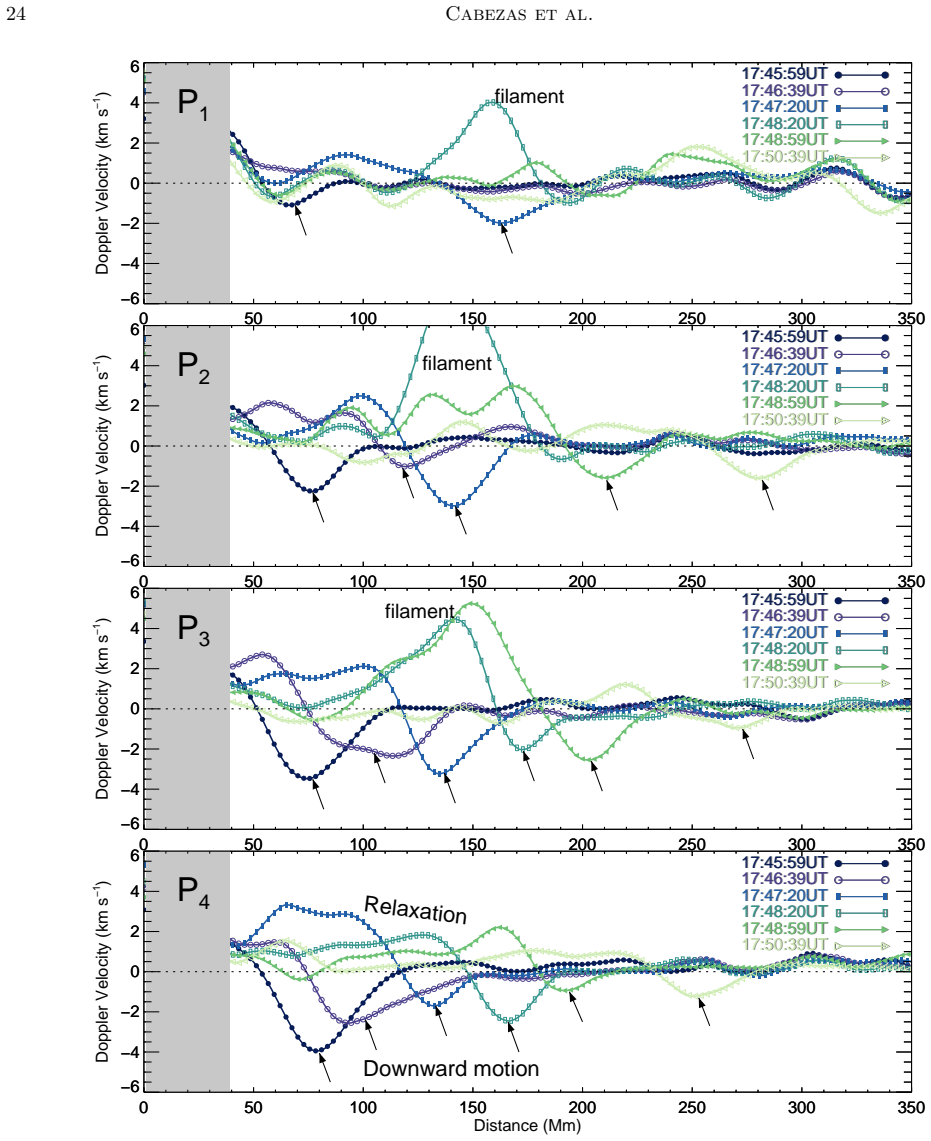
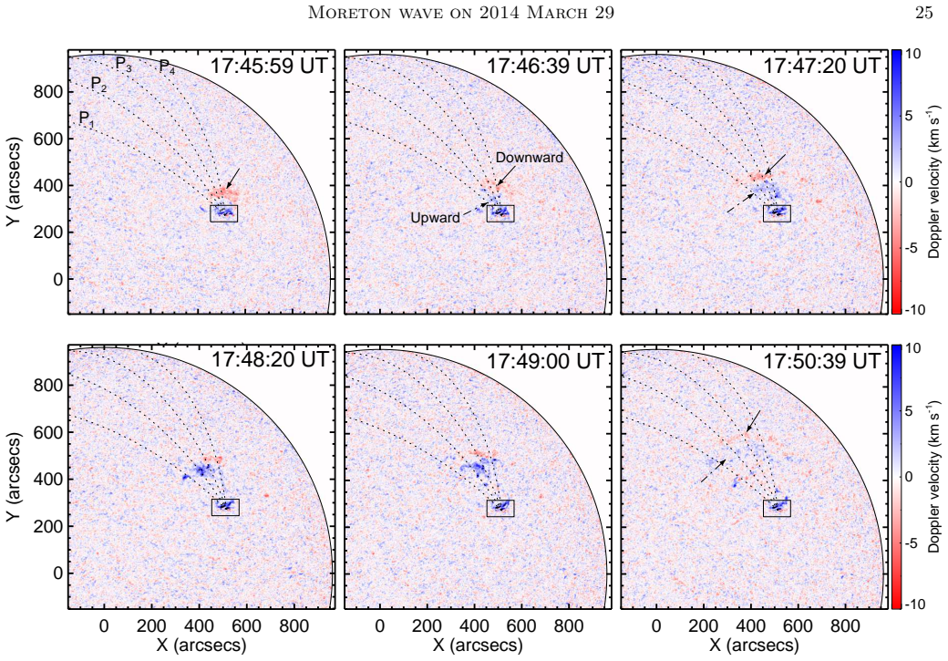
The central claim is that the Moreton wave of 2014 March 29 was the chromospheric footprint of a weak, almost perpendicular fast-mode shock propagating in the corona. In H-$\alpha$ wing data the leading edge appears as a red-wing absorption and blue-wing brightening, which the paper calibrates through a synthetic Doppler signal into a downward line-of-sight velocity reaching $-4$ km/s, with a delayed upward swing. Using the momentum- and energy-flux matching at the corona–chromosphere boundary and the weak-shock relation, a 1–4 km/s chromospheric amplitude translates into coronal incident velocities up to about 22 km/s and Mach numbers near 1.1; AIA differential-emission-measure maps give compression ratios that yield the same nearly sonic range ($M_A \approx 1.06$–$1.28$, $M_f \approx 1.05$–$1.27$). The paper therefore claims that a single large-scale MHD disturbance can explain the quasi-simultaneous response of the corona, transition region, and chromosphere, and that the weak shock approximation is sufficient to diagnose coronal shock strength from ground-based H-$\alpha$ Doppler measurements.
Load-bearing premise
The assumption that carries the result is that the H-$\alpha$ Doppler velocity at the wave front equals the transmitted velocity amplitude $v_t$ of a one-dimensional hydrodynamic shock crossing the transition region, with a density ratio $a=\rho_{\mathrm{ch}}/\rho_{\mathrm{co}} \approx 100$ and a negligible sound-speed ratio; if projection or brightness effects contaminate the H-$\alpha$ signal, the derived Mach numbers shift.
Editorial extensions
If this is right
- If the central claim is right, Moreton-wave Doppler amplitudes can be used as a ground-based measure of coronal shock Mach number without EUV data.
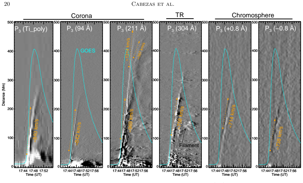
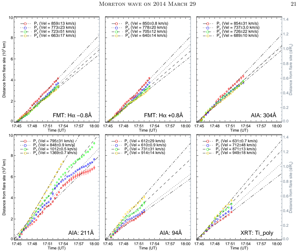
- The observed propagation speeds (640–859 km/s in H-alpha, faster along some coronal paths) imply that the shock strength and direction are shaped by the local Alfvén speed, favoring propagation into weak-field regions.
- The near-simultaneous response in 304 Å, H-alpha, 211 Å, and X-ray data strengthens the standard picture where the chromospheric Moreton wave is the footprint of a globally expanding coronal fast-mode shock.
- The small velocity transmittance (roughly one fifth to one quarter) quantifies why only weak chromospheric Doppler signatures are seen even when the coronal disturbance is large.
- For this event the shock is weak ($M_A, M_f \lesssim 1.3$), so the weak-shock approximation is internally consistent.
Reading between the lines
- A testable extension: compare these Mach numbers with type II radio-burst drift speeds for the same event; agreement would confirm the weak-shock mapping, while systematic disagreement would point to projection or non-Doppler contamination in the H-alpha signal.
- The same Doppler-signal method applied to other Moreton waves observed with H-alpha wing telescopes could produce a statistical sample of coronal shock strengths and their dependence on flare energy.
- Because the H-alpha wings at $\pm 0.8$ Å sample a fixed wavelength, line-profile broadening or intensity changes can masquerade as Doppler shift; full-profile spectroscopy at the wave front would separate true mass motion from thermodynamic changes.
- If the direction-dependence of the wave speed reflects the Alfvén-speed map, Moreton-wave kinematics themselves could be inverted to constrain coronal magnetic-field topology in the low corona.
Signed reviews
Editorial analysis
A structured set of objections, weighed in public.
Referee Report
Summary. The paper reports a multiwavelength study of the Moreton wave associated with the X1.0 flare on 2014 March 29, using Flare Monitoring Telescope Hα wing observations, SDO/AIA EUV data, and Hinode/XRT. The authors measure the Moreton wave propagation speed (640–859 km/s) and, from Hα wing Doppler signals, infer a maximum downward chromospheric velocity of about 4 km/s at the wave front. They then use a weak-shock transmission model to convert this chromospheric velocity amplitude into an incident-shock Mach number in the corona, and independently derive Alfvén and fast-mode Mach numbers from AIA-based differential emission measure compression ratios. The two diagnostics yield overlapping Mach number ranges (Hα: up to ~1.12; DEM: 1.05–1.27), which the authors interpret as consistent evidence for a weak fast-mode shock.
Significance. If the results stand, the paper provides a valuable multi-diagnostic case study of a Moreton wave: it quantifies the chromospheric velocity amplitude with Hα wing imaging, derives shock Mach numbers from two independent datasets, and connects the chromospheric and coronal signatures of a global disturbance. The use of the FMT wing data to extract Doppler velocities and the combination with DEM analysis are genuine strengths. The paper also carefully discusses limitations such as line-of-sight projection and the restricted DEM temperature range. However, the derivation of the central transmission relation contains an algebraic error that must be corrected before the quantitative results can be accepted.
major comments (3)
- [§5.1, Eq. (4)] Equation (4) is not correctly derived from Eqs. (2) and (3). Dividing Eq. (3) by Eq. (2) gives vi = [1 + a(cch/cco)] vt / 2, not vi = [(1 + sqrt(a))/2] vt. The printed form holds only under the unstated assumption cch/cco = 1/sqrt(a). Using the paper's own values (cch = 10 km/s, cco = 185 km/s, a = 100), the coefficient is about 3.2, not 5.5, so the incident velocities vi in Table 2 and the velocity-transmittance discussion in §6.3 and Figure 14 are overestimated by a factor of about 1.7. Please correct Eq. (4), Table 2, Figure 14, and all related text, or explicitly state and justify the additional assumption on the sound-speed ratio.
- [§5.1 vs. §5.2] The treatment of the sound-speed ratio cch/cco is internally inconsistent. In §5.2 the term cch/cco is neglected as small in Eq. (5), but Eq. (4) as printed effectively requires cch/cco = 1/sqrt(a) ≈ 0.1, which is not negligible. With the stated chromospheric and coronal sound speeds (10 and 185 km/s), cch/cco ≈ 0.054, so neglecting it in Eq. (5) is reasonable, but the same ratio cannot also be set to 0.1 in Eq. (4). The manuscript should reconcile these two approximations and state which values of cch and cco are used in each relation.
- [§5.2, Eq. (5) and Table 3] The Hα-based Mach numbers in Table 3 are computed from Eq. (5) using the observed vt, not from Eq. (4). Therefore the algebraic error in Eq. (4) does not directly invalidate the Hα Mach numbers. However, the strong claim of consistency with the DEM-derived Mach numbers rests entirely on the validity of Eq. (5), which assumes a one-dimensional, purely hydrodynamic weak shock with the transition region approximated as a contact discontinuity. The paper should explicitly state the regime of validity of this approximation and discuss how neglecting magnetic fields and the oblique nature of the shock could affect the derived Mach numbers, in order to support the cross-diagnostic comparison.
minor comments (4)
- [General] There are several typographical errors, e.g., 'does exit' in the introduction should be 'does exist', and 'Filter trasmission' in Figure 7 should be 'Filter transmission'.
- [§5.3, Eq. (8)] Equation (8) assumes that the line-of-sight depth l is the same ahead of and behind the shock, and that the proton number density is constant along the line of sight. The paper should explicitly note that this is an approximation and comment on how inhomogeneities or temperature-dependent filling factors might bias the compression ratio.
- [§4.2 and Figure 8] The Doppler velocities are line-of-sight velocities, but the event is at N11, W32, so the radial (vertical) component is foreshortened. The paper does not discuss this projection effect or its impact on the maximum downward velocity of 4 km/s; a brief quantitative statement would be useful.
- [§5.3 and Figure 13] The Mach numbers derived from the DEM compression ratio are presented without error bars or uncertainties. Since the compression ratio X enters through Eq. (7) nonlinearly, it would clarify the robustness of the quoted ranges (1.06–1.28 and 1.05–1.27) if some estimate of the uncertainty from the DEM inversion and the choice of β were provided.
Circularity Check
No load-bearing circularity: H-alpha and DEM Mach numbers come from independent observables; the apparent Eq. (4) algebra error is a correctness issue, not a circular reduction; only a minor non-load-bearing self-citation (Takahashi et al. 2015) exists.
full rationale
The paper's central claim is the mutual consistency of two diagnostics of the same coronal shock. The H-alpha branch measures vt = 4 km/s with an FMT Doppler calibration (Sec. 4), then converts it to an incident-shock Mach number through the weak-shock Rankine-Hugoniot relation Eq. (5), using only cch = 10 km/s, gamma = 5/3, and the small-ratio approximation cch/cco << 1. No DEM-derived quantity enters this branch. The DEM branch measures EM before/behind the front, forms X via Eq. (8), adopts T1 = 2.5 MK and vA = 768 km/s from XRT, and solves Eq. (7) for MA and Eq. (9) for Mf. No H-alpha velocity enters this branch. The parameters a = 100, the DEM temperature window 6.1 <= log T/K <= 6.4, and beta = 0.06 are inputs chosen from observations or standard atmospheric values, not fitted to make the two Mach-number sets agree. Hence the agreement (H-alpha Mi ~ 1.02-1.12; DEM MA ~ 1.06-1.28, Mf ~ 1.05-1.27) is not constructed. The only self-citation of note is 'Similar to Takahashi et al. (2015)' for Eq. (4); Takahashi et al. includes two co-authors, but the relation is also re-derived in the text and the paper's Mach-number estimate does not use Eq. (4). Separately, Eq. (4) as printed does not follow from Eqs. (2)-(3) unless cch/cco = 1/sqrt(a), and with the paper's own cch = 10 km/s and cco = 185 km/s the coefficient would be 3.2 rather than 5.5; this is an internal algebra/correctness problem, not a circularity, and the central consistency argument rests on Eq. (5) and DEM, which are unaffected. The paper also states its own limitations (1D hydrodynamic, no magnetic field effects in Sec. 5.2; DEM restricted to log T 6.1-6.4), which further shows the derivations are not being forced to an externally predetermined answer.
Assumptions & free parameters
free parameters (3)
- Density ratio a = ρ_ch/ρ_co =
≈100
- DEM temperature range =
6.1 ≤ log T/K ≤ 6.4
- Chromospheric sound speed c_ch =
≈10 km/s
assumptions (5)
- domain assumption The transition region can be modeled as a contact discontinuity in a 1D hydrodynamic Riemann problem, and the H-alpha Doppler velocity equals the transmitted velocity amplitude vt.
- standard math Weak shock approximation (M_i^2 - 1 << 1) is valid for the coronal and chromospheric shocks.
- domain assumption The emission measure ratio gives the compression ratio via X = sqrt(EM2/EM1) with constant path length l.
- domain assumption The mean propagation speed of the X-ray wave (790 km/s) represents the fast-mode speed in the corona.
- standard math The MHD oblique shock jump relation (Eq. 6) from Priest (2000) applies to the observed coronal wave.
Cite this review
Pith. "Pith review of Dynamic Processes of the Moreton Wave on 2014 March 29." pith.science (2026). https://pith.science/paper/R4IQWDVY
@misc{pith2026190803534,
  author       = {Pith},
  title        = {Pith review of: Dynamic Processes of the Moreton Wave on 2014 March 29},
  year         = {2026},
  howpublished = {\url{https://pith.science/paper/R4IQWDVY}},
  note         = {Machine review of arXiv:1908.03534}
}
abstract
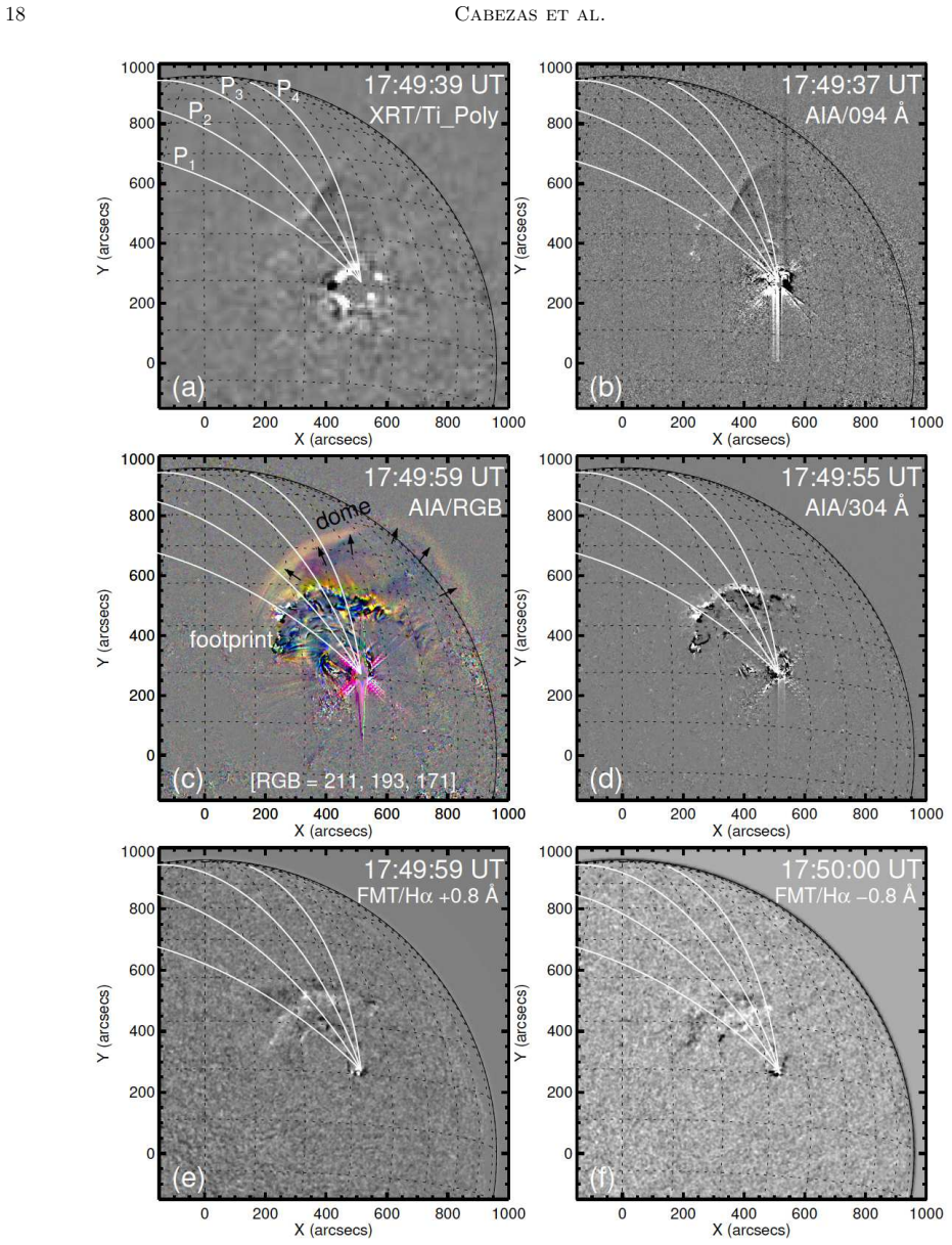
On 2014 March 29, an intense solar flare classified as X1.0 occurred in the active region 12017. Several associated phenomena accompanied this event, among them a fast-filament eruption, large-scale propagating disturbances in the corona and the chromosphere including a Moreton wave, and a coronal mass ejection. This flare was successfully detected in multiwavelength imaging in H-alpha line by the Flare Monitoring Telescope (FMT) at Ica University, Peru. We present a detailed study of the Moreton wave associated with the flare in question. Special attention is paid to the Doppler characteristics inferred from the FMT wing (H-alpha$\pm0.8$~{\AA}) observations, which are used to examine the downward/upward motion of the plasma in the chromosphere. Our findings reveal that the downward motion of the chromospheric material at the front of the Moreton wave attains a maximum velocity of 4 km/s, whereas the propagation speed ranges between 640 and 859 km/s. Furthermore, utilizing the weak shock approximation in conjunction with the velocity amplitude of the chromospheric motion induced by the Moreton wave, we derive the Mach number of the incident shock in the corona. We also performed the temperature-emission measure analysis of the coronal wave based on the Atmospheric Imaging Assembly (AIA) observations, which allowed us to derive the compression ratio, and to estimate the Alfv\'en and fast-mode Mach numbers of the order of 1.06-1.28 and 1.05-1.27. Considering these results and the MHD linear theory we discuss the characteristics of the shock front and the interaction with the chromospheric plasma.
Figures


Figures from the paper (12 more)




Reference graph
Works this paper leans on
-
[1]
-VGCU?<rl=Q^
thebibliography [1] 20pt to REFERENCES 6pt =0pt 10pt plus 3pt =0pt =0pt =1pt plus 1pt =0pt =0pt -12pt =13pt plus 1pt =20pt =13pt plus 1pt \@M =10000 =-1.0em =0pt =0pt 0pt =0pt =1.0em @enumiv\@empty 10000 10000 `\.\@m \@noitemerr \@latex@warning Empty `thebibliography' environment \@ifnextchar \@reference \@latexerr Missing key on reference command Each re...
2017
-
[2]
1966, University of Colorado, Boulder (Thesis)
Anderson, G.F. 1966, University of Colorado, Boulder (Thesis)
work page 1966
- [3]
- [4]
- [5]
-
[6]
Balasubramaniam, K.S., Pevtsov, A.A., Neidig, D.F. 2007, , 658, 1379
work page 2007
-
[7]
Balasubramaniam, K.S., Cliver, E.W., Pevtsov, A., et al. 2010, , 723, 587
work page 2010
- [8]
Show all 80 references
-
[9]
& Vourlidas, A
Biesecker, D.A., Myers, D.C., Thompson, B.J., Hammer, D.M. & Vourlidas, A. 2002, , 569, 1009
2002
-
[10]
2017, , 836, 33
Cabezas, D.P., Mart\'inez, L.M., Buleje, Y.J., et al. 2017, , 836, 33
2017
-
[11]
T., Shibata, K., Fang, C
Chen, P.F., Wu, S. T., Shibata, K., Fang, C. 2002, , 572, L99
2002
-
[12]
2005, , 622, 1202
Chen, P.F., Fang, C., Shibata, K. 2005, , 622, 1202
2005
-
[13]
2005, , 121, 201
Chen, P.F., Ding, M.D., Fang, C. 2005, , 121, 201
2005
-
[14]
2016, Low-Frequency Waves in Space Plasmas, Monograph Series, 216, 381
Chen, P.F. 2016, Low-Frequency Waves in Space Plasmas, Monograph Series, 216, 381
2016
-
[15]
2015, , 807, 143
Cheung, M.C., Boerner, P., Schrijver, C.J. 2015, , 807, 143
2015
-
[16]
E., et al
Delaboudini\` e re, J.-P., Artzner, G. E., et al. 1995, , 162, 291
1995
-
[17]
1999, , 190, 107
Delann\' e e, C., Aulanier, G. 1999, , 190, 107
1999
-
[18]
2000, , 545, 512
Delann\' e e, C. 2000, , 545, 512
2000
-
[19]
1968, , 4, 229
Dodson, H.W., Hedeman, E.R. 1968, , 4, 229
1968
-
[20]
Domingo, V., Fleck, B., Poland, A. I. 1995, , 162, 1
1995
-
[21]
2002, , 54, 481
Eto, S., Isobe, H., Narukage, N., et al. 2002, , 54, 481
2002
-
[22]
2016, , 291, 3217
Francile, C., L\'opez, F.M., Cremades, H. 2016, , 291, 3217
2016
-
[23]
2004, , 610, 572
Gilbert, H.R., Thomas, E.H. 2004, , 610, 572
2004
-
[24]
2007, , 243, 63
Golub, L., Deluca, E., Austin, G., et al. 2007, , 243, 63
2007
-
[25]
1999, , 187, 229
Handy, B.N., Acton, L.W., Kankelborg, C.C., et al. 1999, , 187, 229
1999
-
[26]
2003, , 587, 429
Harra, L.K., Sterling, A.C. 2003, , 587, 429
2003
-
[27]
2011, , 737, L4
Harra, L.K., Sterling, A.C., G\" o m\" o ry P., Veronig, A. 2011, , 737, L4
2011
-
[28]
2003, , 212, 121
Hudson, H., Khan, J.I., Lemen, J.R., Nitta, N.V., Uchida, Y. 2003, , 212, 121
2003
-
[29]
2017, , 292, 63
Ichimoto, K., Ishii, T.T., Otsuji K., Kimura, G., et al. 2017, , 292, 63
2017
-
[30]
1970, , 11, 310
Kai, K. 1970, , 11, 310
1970
-
[31]
Khan, J.I., Aurass, H., 2002, , 1018, 1031
2002
-
[32]
2000, , 141, 357
Klassen A., Aurass, H., Mann, G., Thompson, B.J. 2000, , 141, 357
2000
-
[33]
2015, , 806, 9
Kleint, L., Battaglia, M., Reardon, K., et al. 2015, , 806, 9
2015
-
[34]
2007, , 243, 3
Kosugi, T., Matsuzaki, K., Sakao, T., et al. 2007, , 243, 3
2007
-
[35]
et al., 1995, JGG, 47, 1043
Kurokawa, H., Ishiura, K., Kimura, G. et al., 1995, JGG, 47, 1043
1995
-
[36]
1987, Fluid Mechanics 2nd ed., (Pergamon Press)
Landau, L.D., Lifshitz, E.M. 1987, Fluid Mechanics 2nd ed., (Pergamon Press)
1987
-
[37]
R., Title, A., Akin, D
Lemen, J. R., Title, A., Akin, D. J., et al. 2012, , 275, 17
2012
-
[38]
2010, , 723, L53
Liu, W.L., Nitta, N.V., Schrijver, C.J., et al. 2010, , 723, L53
2010
-
[39]
2014, , 289, 3233
Liu, W., Ofman. 2014, , 289, 3233
2014
-
[40]
2018, , 864, L24
Liu, W., Jin, M., Downs, C., Ofman, L., et at. 2018, , 864, L24
2018
-
[41]
2016, , 297, 7
Long, D.M., Bloomfield, D.S., Chen, P.F., et al. 2016, , 297, 7
2016
-
[42]
2019, ArXiv e-prints
Long, D.M., Jenkins, J., & Valori, G. 2019, ArXiv e-prints
2019
-
[43]
1963, Structure and Development of Solar Active Regions, IUA Symp., 35, 485, (K.O
Meyer, F. 1963, Structure and Development of Solar Active Regions, IUA Symp., 35, 485, (K.O. Kiepenhever)
1963
-
[44]
Moreton, G. E. 1960, , 65, 494
1960
-
[45]
E., Ramsey, H
Moreton, G. E., Ramsey, H. E. 1960, , 72, 357
1960
-
[46]
& Kurokawa, H
Morimoto, T. & Kurokawa, H. 2003a, , 55, 503
-
[47]
& Kurokawa, H
Morimoto, T. & Kurokawa, H. 2003b, , 55, 1141
-
[48]
Morimoto, T., Kurokawa, H., Shibata, K., Ishii, T. T. 2010, , 62, 939
2010
-
[49]
2010, , 708, 1639
Muhr, N., Vr s nak, B., Temmer, M., Veronig, A.M., Magdaleni\' c , J. 2010, , 708, 1639
2010
-
[50]
2014, , 289, 4563
Muhr, N., Veronig, A.M., Kienreich, I.W., Vr s nak, B., Temmer, M., Bein, B.M. 2014, , 289, 4563
2014
-
[51]
2002, , 572, L109
Narukage, N., Hudson, H.S., Morimoto, T., et al. 2002, , 572, L109
2002
-
[52]
2004, , 56, L5
Narukage, N., Moritmoto T., Kadota, M., et al. 2004, , 56, L5
2004
-
[53]
2008, , 684, L45
Narukage, N., Ishii, T.T., Nagata, S., UeNo., S., et al. 2008, , 684, L45
2008
-
[54]
2011, , 269, 169
Narukage, N., Sakao, T., Kano, R., et al. 2011, , 269, 169
2011
-
[55]
2013, , 776, 58
Nitta, N.V., Schrijver, C.J., Title, A.M., Liu, W. 2013, , 776, 58
2013
-
[56]
2014, , 289, 1257
Nitta, N.V., Aschwanden, M.J., Freeland, S.L. 2014, , 289, 1257
2014
-
[57]
D., Thompson, B
Pesnell, W. D., Thompson, B. J., Chamberlin, P. C. 2012, , 275, 3
2012
-
[58]
Priest, E. R. 2000, Solar Magnetohydrodynamics (Dordrecht: Reidel)
2000
-
[59]
Shibata, K., Kitai, R., Katoda, M., et al., 2011, Solar Activity in 1992-2003, (Kyoto: Kyoto University Press)
2011
-
[60]
1976, Solar Flares (Dordrecht: Reidel)
S vestka, Z. 1976, Solar Flares (Dordrecht: Reidel)
1976
-
[61]
2015, , 801
Takahashi, T., Asai, A., Shibata, K. 2015, , 801
2015
-
[62]
J., Gurman, J
Thompson, B. J., Gurman, J. B., Neupert, W. M., et al. 1999, , 517, L151
1999
-
[63]
J., Myers, D.C
Thompson, B. J., Myers, D.C. 2009, , 183, 225
2009
-
[64]
1968, , 4, 30
Uchida, Y. 1968, , 4, 30
1968
-
[65]
1973, , 28, 495
Uchida, Y., Altschuler, M., Newkirk, G. 1973, , 28, 495
1973
-
[66]
2007, Bull
UeNo, S., Shibata, K., Kimura, G., Nakatani, Y., Kitai, R., Nagata, S. 2007, Bull. Astr. Soc. India, 35, 697
2007
-
[67]
Vanninathan, K., Veronig, A.M., Dissauer, K., et al., 2015, , 812, 173
2015
-
[68]
2006, , 647, 1466
Veronig, A.M., Temmer, M., Vr s nak, B., Thalmann, J. 2006, , 647, 1466
2006
-
[69]
M., G\" o m\" o ry P., Kienreich, I
Veronig, A. M., G\" o m\" o ry P., Kienreich, I. W., , 743, L10
-
[70]
Vr s nak, B., Warmuth, A., Braj s a, R., Hanslmeier, A., 2002a, , 394, 299
-
[71]
2002b, , 396, 673
Vr s nak, B., Magdaleni\' c , J., Aurass, H., & Mann, G. 2002b, , 396, 673
-
[72]
Vr s nak, B., Magdaleni\' c , J., Temmer, T., et al., 2005, , 625, L67
2005
-
[73]
2016, , 219, 89
Vr s nak, B., Z ic, T., Luli\'c, S., Temmer, M., Veronig, A.M. 2016, , 219, 89
2016
-
[74]
2001, , 560, L105
Warmuth, A., Vr s nak, B., Aurass, H., Hanslmeier, A. 2001, , 560, L105
2001
-
[75]
2004, , 418, 1117
Warmuth, A., Vr s nak, B., Magdaleni\' c , J., Hanslmeier, A., Otruba, W. 2004, , 418, 1117
2004
-
[76]
2005, , 626, L121
Warmuth A., Mann, G., and Aurass, H. 2005, , 626, L121
2005
-
[77]
2015, LRSP, 12, 3
Warmuth, A. 2015, LRSP, 12, 3
2015
-
[78]
Wills-Davey, M.J., Thompson, B.J., 1999, , 190, 467
1999
-
[79]
2001, , 372, 676
Zhang, H. 2001, , 372, 676
2001
-
[80]
2011, , 63, 685
Zhang, Y., Kitai, R., Narukage, Y., et al. 2011, , 63, 685
2011
Reviewed August 14, 2026 · model on record in the stance chip above.
Discussion (0). Continue with ORCID to comment.