REVIEW 3 major objections 5 minor 28 references
Real-Time Gradient Waveform Design for Arbitrary $k$-Space Trajectories
T0 review · 3 major / 5 minor · reviewed 2026-08-06 · deepseek-v4-flash
Pith's one-line read A recursive solver designs MRI gradient waveforms in real time for any k-space trajectory.
desk verdict A clearly specified recursive gradient solver that is genuinely fast and matches the optimal-control reference on seven trajectories, but the 'arbitrary trajectory, hardware-compliant' claim rests on a slew-rate guarantee that the final secant reparameterization does not actually provide. read the letter →
The pith
A machine-rendered reading of the paper's core claim, the machinery that carries it, and where it could break.
The reading
What carries the argument
The load-bearing object is the per-step quadratic equation that selects the next gradient vector. Writing the next gradient as a unit vector along the local trajectory tangent times a magnitude m, the slew-rate constraint ||m g_hat - g(t_this)|| <= S_lim $\Delta$ t expands to a quadratic in m; its farthest root, capped by G_lim and by the curvature escape velocity $\sqrt$(S_lim/kappa), is the time-optimal magnitude. The DTFBS strategy runs this recursion forward and backward and keeps the pointwise minimum, which guarantees the magnitude stays below the curvature limit so the quadratic always has a real root. A piecewise cubic spline reparameterization gives the C2 trajectory derivatives needed for the tangent and curvature, and the final waveform is the finite difference of the spline at hardware time samples, with temporal oversampling factor R_samp=8 chosen to keep slew-rate overshoot below about 0.1 percent.
What would settle it
Take the published solver with R_samp=8 and feed it a deliberately non-smooth or high-curvature trajectory—for example, a path with a sharp corner or a random-walk spline whose curvature exceeds the tested Spiral values—then compute the true slew rate of the final finite-difference waveform at the hardware temporal resolution. If the maximum slew-rate magnitude exceeds S_lim by more than the small tolerance the paper reports for ordinary trajectories, the claim that the method is real-time and hardware-compliant for arbitrary trajectories is falsified for that class of inputs.
Extended reading notes
Core claim
On its own terms, the paper establishes that time-optimal, hardware-compliant gradient waveforms for an arbitrary k-space trajectory can be computed recursively in constant time per step, in one non-iterative pass. The key reduction is that the two local constraints—the gradient magnitude limit and the slew-rate limit—become, together with the trajectory-tangent direction condition, the intersection of a ray with a Euclidean ball, whose farthest point is given by the positive root of a quadratic. The recursion is kept feasible by capping the gradient magnitude at the escape velocity sqrt(S_lim/kappa) set by local curvature, and by taking the pointwise minimum of a forward sweep and a backward sweep, the Discrete-Time Forward and Backward Sweep. A cubic-spline reparameterization of the trajectory supplies the C2 derivatives the recursion needs, and the final gradient is recomputed as the finite difference of trajectory samples to preserve the commanded k-space path. Measured against the standard optimal-control method on seven trajectories, the paper reports roughly a tenfold reduction in recursive steps, computation times of about 1–2 ms that are always below the gradient duration, slew-rate overshoot below 0.05 percent, and matching gradient durations, together with phantom and in vivo images that show no visible distortion.
Load-bearing premise
The method assumes that solving with a fixed temporal oversampling factor R_samp=8 and then replacing the gradients by finite differences of the spline yields a final waveform whose slew rate stays within the hardware limit for every input trajectory, including high-curvature or non-smooth ones; the paper itself notes this reparameterization 'may lead to a trade-off in slew-rate accuracy' and selects R_samp from one Spiral test case.
Editorial extensions
If this is right
- Gradient computation moves from the pre-scan stage to the scan stage: the solver finishes before the gradient it computes has finished playing out, so non-Cartesian scans no longer wait for a multi-second or multi-minute design step.
- Trajectory design is freed from a small set of precomputed interleaf shapes; each interleaf can in principle have a unique shape because the waveform is computed on the fly.
- Scan-time adaptation becomes possible: changing the trajectory, the gradient limit, or the slew-rate limit (for example, in cardiac or pediatric imaging) can be followed by an immediate recomputation of the waveform.
- The substantial reduction in slew-rate overshoot—from about 4 percent to below 0.05 percent in the reported benchmarks—lowers the risk of scan failure due to gradient hardware violations.
Reading between the lines
- Because the solver is non-iterative and runs in O(N) with a small constant, it could serve as the inner loop of trajectory-optimization searches that currently treat gradient feasibility as a separate expensive step; that use is not explored in the paper.
- The chosen R_samp=8 was tuned on a Spiral trajectory; a systematic sweep over high-curvature or non-smooth inputs would show whether a fixed oversampling factor, rather than an error-based adaptive one, is enough to keep the secant-based final waveform within slew-rate limits for truly arbitrary paths.
- The real-time claim is tied to the tested CPU; porting the recursion to GPU or FPGA hardware would likely push computation well below one millisecond and make the method compatible with even shorter readout gradients.
- A formal bound connecting spline curvature, R_samp, and worst-case slew-rate error would turn the empirical overshoot numbers into a guarantee; the paper currently provides only experimental evidence.
Editorial analysis
A structured set of objections, weighed in public.
Referee Report
Summary. The manuscript proposes a recursive, non-iterative method for designing gradient waveforms for arbitrary k-space trajectories. The method computes each next gradient vector from the slew-rate and maximum-gradient constraints together with a tangency constraint, updates the trajectory parameter with an RK2 step, and adds three preprocessing/postprocessing components: a Discrete-Time Forward and Backward Sweep (DTFBS) intended to guarantee existence of the quadratic solution, a cubic-spline reparameterization to supply C2 trajectory derivatives, and a finite-difference reparameterization of the output gradients to preserve trajectory fidelity. The authors report experiments on seven non-Cartesian trajectories with 100 repetitions each, comparing computation time, output duration, and slew-rate overshoot against the optimal-control method of Lustig et al. They find near-identical output durations, computation time shorter than gradient duration for all tested trajectories, a >89% reduction in computation time, and a >98% reduction in slew-rate overshoot. Phantom and in vivo imaging with the generated waveforms is presented.
Significance. If the central claims hold, the method is a practically valuable contribution: it would move non-Cartesian gradient design from the pre-scan stage into real time, enable per-interleaf trajectory design, and substantially reduce slew-rate overshoot relative to the dominant optimal-control approach. The paper's empirical work is a genuine strength: seven trajectory classes, 100-run statistics, an external baseline comparison, detailed computation-time measurements, a linear-complexity check with R2=0.9996, and imaging validation support the engineering claims. The reported output durations agree with the Lustig reference without fitting, which is the right kind of evidence for time-optimality. However, the central guarantee of hardware compliance for arbitrary trajectories is not established by the derivations; it rests on an empirical extrapolation from seven trajectories and on a fixed temporal oversampling factor selected from one trajectory. The DTFBS feasibility argument is also asserted rather than proved. These gaps are load-bearing for the abstract's unqualified claims of 'hardware-compliant' and 'arbitrary k-space trajectories'.
major comments (3)
- [II-G, Eq. (21)] The final delivered gradient waveform is not the recursively solved sequence that satisfies the slew-rate constraint; it is the secant g(t_i) = (k(t_{i+1}) - k(t_i))/Δt of the fitted spline, evaluated after downsampling. The recursive solver guarantees ∥g(t_next)-g(t_this)∥ ≤ S_lim Δt for the sequence defined by Eq. (13), but no bound is derived for the second differences of the spline samples, so the slew rate of the final hardware waveform can in principle exceed S_lim even when the solver's internal sequence is compliant. Section II-G explicitly acknowledges a 'trade-off in slew-rate accuracy', and Section IV-C selects R_samp=8 from a single Spiral trajectory (Fig. 2D). This does not support the abstract's unqualified claim that the method is hardware-compliant for arbitrary trajectories. A worst-case error bound depending on R_samp, spline derivatives, and trajectory curvature, or a conservative final projection/clipping step with a proof of convergence, is needed.
- [II-E, Eqs. (15)-(18)] The DTFBS feasibility argument is asserted intuitively rather than proved. Equation (15) takes the minimum of the forward and backward solutions, but no proof is given that the pointwise minimum preserves the slew-rate constraint when the forward sweep switches to the backward envelope, and the linear interpolation used to evaluate g_back(p) in the forward sweep can itself create a slew-rate violation. Additionally, the escape-velocity throttle G_esc = sqrt(S_lim/κ) is introduced without a proof that it guarantees Eq. (12) has a real root for all parameter updates generated by the RK2 step in Eq. (14). Because the existence of the recursive solution is a central methodological claim, this needs either a rigorous proof or a concrete counterexample that motivates a different existence mechanism.
- [IV-C and Table II] The choice R_samp=8 is justified by a single experiment on one Spiral trajectory, while the paper's general claims cover arbitrary trajectories with widely varying curvature and smoothness. Table II shows that for the seven tested trajectories the achieved slew-rate overshoot is at most 0.050%, but this is an empirical statement about those inputs, not a guarantee for the class of arbitrary k-space trajectories. The manuscript should either provide a transferable bound on the final slew-rate error as a function of R_samp and trajectory properties, or explicitly restrict the 'arbitrary trajectory' claim to trajectories for which such a bound is verified.
minor comments (5)
- [Eq. (25)] The notation s[i] in the definition of E_slew is ambiguous because s(t) was previously defined as a vector; please state explicitly that s[i] denotes the magnitude ∥g(t_i)-g(t_{i-1})∥/Δt.
- [Section II-D, Eq. (11)] The sign term sgn(dp/dt) is used before the recursive update of p is described; please clarify how the traversal direction is initialized and whether the sign is guaranteed to remain consistent for self-intersecting trajectories.
- [Section IV-B and Fig. 2C] The linear-complexity claim would be more informative if the fitted slope and intercept were reported, since the intercept is relevant for assessing whether the method remains real-time for very short gradient waveforms.
- [Section IV-C] The statement that 'E_slew decreases exponentially with increasing R_samp' is supported by only one trajectory; please label the curve as trajectory-specific or add error bars/other trajectories.
- [Section IV-D] The time-optimality conclusion is drawn from equality of T_grad with the Lustig implementation on seven trajectories; reporting the matching tolerance and the discretization error of the reference method would make the claim more precise.
Circularity Check
No circularity: the recursive solver's constraints, external optimal-control benchmark, and measured runtime comparisons carry the argument; the R_samp choice is hyperparameter tuning, not a fitted prediction.
full rationale
The derivation chain is self-contained. The recursive solver (Eqs. 7-13) enforces per-step gradient and slew constraints and greedily maximizes the next gradient magnitude; the DTFBS step (Eqs. 15-18) takes minima of forward/backward solutions to maintain feasibility. These are construction steps, not predictions. Time-optimality is validated against Lustig's external optimal-control method [13] (duration columns in Table II), and the reported T_grad values agree without fitting any parameter to those durations. Computation-time and slew-overshoot reductions are measured outputs, not imposed identities. The one tunable parameter, R_samp, is selected in Section IV-C from a Spiral trade-off curve and then applied to all trajectories; this is ordinary hyperparameter selection rather than a prediction forced by construction. The acknowledged Section II-G trade-off, "the preferred approach may lead to a trade-off in slew-rate accuracy," means the final finite-difference waveform is not slew-compliant by construction, but that is a correctness/robustness limitation, not circular reasoning, and the paper discloses it. No load-bearing self-citation or imported uniqueness theorem appears; the only external load-bearing reference is Lustig's independent optimal-control formulation, against which the method is benchmarked. Therefore no circular step is present.
Assumptions & free parameters
free parameters (2)
- Temporal oversampling factor R_samp =
8
- Spline sample count N =
not specified
assumptions (5)
- domain assumption The gradient field varies linearly between adjacent temporal samples (Section II-C).
- domain assumption The tangent at the next trajectory sample is approximately equal to the tangent at the current sample (Eq. 9).
- ad hoc to paper The minimum of the forward and backward sweep solutions is a feasible trajectory satisfying the slew-rate constraint (Eq. 15).
- ad hoc to paper A fixed temporal oversampling factor R_samp=8 keeps the finite-difference reparameterized gradient within the slew-rate limit for arbitrary trajectories (Section IV-C).
- domain assumption Cubic spline interpolation through sampled trajectory points preserves the original trajectory shape sufficiently (Section II-F).
Cite this review
Pith. "Pith review of Real-Time Gradient Waveform Design for Arbitrary $k$-Space Trajectories." pith.science (2026). https://pith.science/paper/RDQMJ2V2
@misc{pith2026250721625,
  author       = {Pith},
  title        = {Pith review of: Real-Time Gradient Waveform Design for Arbitrary $k$-Space Trajectories},
  year         = {2026},
  howpublished = {\url{https://pith.science/paper/RDQMJ2V2}},
  note         = {Machine review of arXiv:2507.21625}
}
abstract
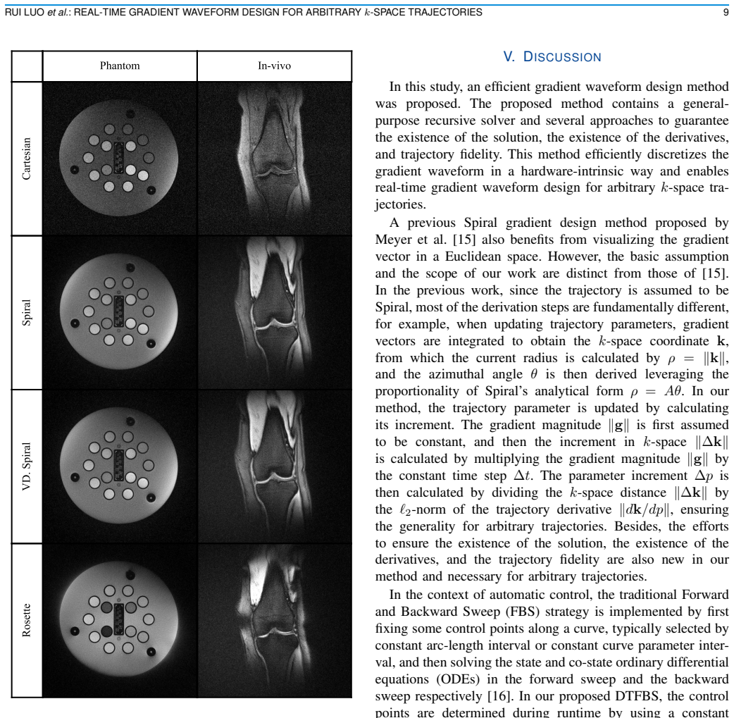
\textbf{Objective: }To develop a real-time method for designing gradient waveforms for arbitrary $k$-space trajectories that are time-optimal and hardware-compliant. \textbf{Methods: }The gradient waveform is solved recursively under both the slew-rate and the trajectory constraints. The gradient constraint is enforced by thresholding the $\ell_2$-norm of the next gradient vector. The constraints form a quadratic equation. To ensure the existence of the solution, a novel Discrete-Time Forward and Backward Sweep (DTFBS) strategy is proposed. To ensure the existence of the trajectory derivatives, the trajectory function is reparameterized as a piecewise cubic polynomial function with $C^2$ continuity. To ensure trajectory fidelity, the output gradient waveform is reparameterized by the finite difference of the trajectory samples. Simulation experiments across seven commonly adopted non-Cartesian trajectories were conducted to validate generality, time-optimality, real-time capability, slew-rate accuracy, and improvements over prior work. Imaging feasibility of the designed time-optimal gradient waveform was validated in phantom and in vivo experiments. \textbf{Results: }The proposed method achieves a $>89\%$ reduction in computation time and simultaneously reduces slew-rate overshoot by $>98\%$ compared to the prior method across all involved trajectories. The computation time of the proposed method is shorter than the gradient duration for all tested cases, validating the real-time capability of the proposed method. \textbf{Conclusions: }The proposed method enables real-time and hardware-compliant gradient waveform design, achieving significant reductions in computation time and slew-rate overshoot compared to the previous method. \textbf{Significance: }This is the first method achieving real-time gradient waveform design for arbitrary $k$-space trajectories.
Figures


Figures from the paper (3 more)


Reference graph
Works this paper leans on
-
[1]
High-speed spiral-scan echo planar nmr imaging-i,
C. B. Ahnet al., “High-speed spiral-scan echo planar nmr imaging-i,” IEEE Trans. Med. Imag., vol. 5, no. 1, pp. 2–7, Mar. 1986
work page 1986
-
[2]
Design and analysis of a practical 3d cones trajectory,
P. T. Gurneyet al., “Design and analysis of a practical 3d cones trajectory,”Magn Reson Med, vol. 55, no. 3, pp. 575–582, Mar. 2006
work page 2006
-
[3]
Multishot rosette trajectories for spectrally selective mr imaging,
D. C. Noll, “Multishot rosette trajectories for spectrally selective mr imaging,”IEEE Trans. Med. Imag., vol. 16, no. 4, pp. 372–377, Aug. 1997
work page 1997
-
[4]
Partial fourier shells trajectory for non-cartesian mri,
S. Taoet al., “Partial fourier shells trajectory for non-cartesian mri,” Phys. Med. Biol., vol. 64, no. 4, Feb. 2019
work page 2019
-
[5]
B. M. A. Delattreet al., “Spiral demystified,”Magn Reson Imaging, vol. 28, no. 6, pp. 862–881, Jul. 2010
work page 2010
-
[6]
Three-dimensional mri with an undersampled spherical shells trajectory,
Y . Shuet al., “Three-dimensional mri with an undersampled spherical shells trajectory,”Magn Reson Med, vol. 56, no. 3, pp. 553–562, Sep. 2006
work page 2006
-
[7]
Three-dimensional yarnball k-space acquisition for accelerated mri,
R. W. Stobbe and C. Beaulieu, “Three-dimensional yarnball k-space acquisition for accelerated mri,”Magn Reson Med, vol. 85, no. 4, pp. 1840–1854, Apr. 2021
work page 2021
-
[8]
Efficient 3d low-discrepancy k-space sampling using highly adaptable seiffert spirals,
T. Speidelet al., “Efficient 3d low-discrepancy k-space sampling using highly adaptable seiffert spirals,”IEEE Trans. Med. Imag., vol. 38, no. 8, pp. 1833–1840, Aug. 2019
work page 2019
Show all 28 references
-
[9]
A low-rank deep image prior reconstruction for free-breathing ungated spiral functional cmr at 0.55 t and 1.5 t,
J. I. Hamiltonet al., “A low-rank deep image prior reconstruction for free-breathing ungated spiral functional cmr at 0.55 t and 1.5 t,”Magn Reson Mater Phys Biol Med, vol. 36, no. 3, pp. 451–464, Apr. 2023
2023
-
[10]
Grasp-pro: improving grasp dce-mri through self- calibrating subspace-modeling and contrast phase automation,
L. Fenget al., “Grasp-pro: improving grasp dce-mri through self- calibrating subspace-modeling and contrast phase automation,”Magn Reson Med, vol. 83, no. 1, pp. 94–108, Jan. 2020
2020
-
[11]
Low rank alternating direction method of multipliers reconstruction for mr fingerprinting,
J. Assl ¨anderet al., “Low rank alternating direction method of multipliers reconstruction for mr fingerprinting,”Magn Reson Med, vol. 79, no. 1, pp. 83–96, Jan. 2018
2018
-
[12]
Low rank matrix recovery for real-time cardiac mri,
B. Zhaoet al., “Low rank matrix recovery for real-time cardiac mri,” in2010 IEEE International Symposium on Biomedical Imaging: From Nano to Macro, Apr. 2010, pp. 996–999
2010
-
[13]
A fast method for designing time-optimal gradient waveforms for arbitrary k-space trajectories,
M. Lustiget al., “A fast method for designing time-optimal gradient waveforms for arbitrary k-space trajectories,”IEEE Trans. Med. Imag., vol. 27, no. 6, pp. 866–873, Jun. 2008
2008
-
[14]
Simple but reliable solutions for spiral mri gradient design,
C. Salustriet al., “Simple but reliable solutions for spiral mri gradient design,”J Magn Reson, vol. 140, no. 2, pp. 347–350, Oct. 1999
1999
-
[15]
Rapid method of optimal gradient waveform design for mri,
C. H. Meyer and J. M. Pauly, “Rapid method of optimal gradient waveform design for mri,” US Patent US6 020 739, Feb., 2000
2000
-
[16]
A comparison principle for state-constrained differen- tial inequalities and its application to time-optimal control,
S.-J. Kimet al., “A comparison principle for state-constrained differen- tial inequalities and its application to time-optimal control,”IEEE Trans. Autom. Control, vol. 50, no. 7, pp. 967–983, Jul. 2005
2005
-
[17]
Image reconstruction using a gradient impulse response model for trajectory prediction,
S. J. Vannesjoet al., “Image reconstruction using a gradient impulse response model for trajectory prediction,”Magn Reson Med, vol. 76, no. 1, pp. 45–58, Jul. 2016
2016
-
[18]
Matched-filter acquisition for bold fmri,
L. Kasperet al., “Matched-filter acquisition for bold fmri,”NeuroImage, vol. 100, pp. 145–160, Oct. 2014
2014
-
[19]
A projection algorithm for gradient waveforms design in magnetic resonance imaging,
N. Chauffertet al., “A projection algorithm for gradient waveforms design in magnetic resonance imaging,”IEEE Trans. Med. Imag., vol. 35, no. 9, pp. 2026–2039, Sep. 2016
2026
-
[20]
Fast and robust design of time-optimal k-space trajectories in mri,
M. Davidset al., “Fast and robust design of time-optimal k-space trajectories in mri,”IEEE Trans. Med. Imag., vol. 34, no. 2, pp. 564–577, Feb. 2015
2015
-
[21]
A gradient optimization toolbox for general purpose time-optimal mri gradient waveform design,
M. Loecheret al., “A gradient optimization toolbox for general purpose time-optimal mri gradient waveform design,”Magn Reson Med, vol. 84, no. 6, pp. 3234–3245, Dec. 2020
2020
-
[22]
Optimized diffusion-weighting gradient wave- form design (odgd) formulation for motion compensation and concomi- tant gradient nulling,
O. Pe na-Nogaleset al., “Optimized diffusion-weighting gradient wave- form design (odgd) formulation for motion compensation and concomi- tant gradient nulling,”Magn Reson Med, vol. 81, no. 2, pp. 989–1003, Feb. 2019
2019
-
[23]
Aliasing error of the exp(β √ 1−z 2) kernel in the nonuniform fast fourier transform,
A. H. Barnett, “Aliasing error of the exp(β √ 1−z 2) kernel in the nonuniform fast fourier transform,” Oct. 2020, arXiv:2001.09405
2020 arXiv
-
[24]
A parallel non-uniform fast fourier transform library based on an
A. H. Barnettet al., “A parallel non-uniform fast fourier transform library based on an ”exponential of semicircle” kernel,” Apr. 2019, arXiv:1808.06736
2019 arXiv
-
[25]
Sampling density compensation in mri: Rationale and an iterative numerical solution,
J. G. Pipe and P. Menon, “Sampling density compensation in mri: Rationale and an iterative numerical solution,”Magn Reson Med, vol. 41, no. 1, pp. 179–186, Jan. 1999
1999
-
[26]
K-space trajectory design for reduced mri scan time,
S. Sharmaet al., “K-space trajectory design for reduced mri scan time,” inICASSP 2020 - 2020 IEEE International Conference on Acoustics, Speech and Signal Processing (ICASSP), May 2020, pp. 1120–1124
2020
-
[27]
Cardiac mri: State of the art,
P. S. Rajiahet al., “Cardiac mri: State of the art,”Radiology, vol. 307, no. 3, May 2023
2023
-
[28]
Acoustic noise reduction for spiral mri by gradient derating,
Z. Zhouet al., “Acoustic noise reduction for spiral mri by gradient derating,”Magn Reson Med, vol. 90, no. 4, pp. 1547–1554, Oct. 2023
2023
Reviewed August 6, 2026 · model on record in the stance chip above.
Discussion (0). Sign in to comment.