Power-Linear Polar Directional Fields

Amir Vaxman; Jiabao Brad Wang

REVIEW 4 major objections 4 minor 2 references

Power-Linear Polar Directional Fields

T0 review · 4 major / 4 minor · reviewed 2026-08-07 · deepseek-v4-flash

Challenge this review Re-run · record.json Download PDF Read on arXiv ↗

Pith's one-line read A power-linear polar representation lets users place directional-field singularities on faces, edges, or vertices of a triangle mesh while preserving smoothness.

desk verdict A genuinely new higher-order polar field representation with a smart beveled-mesh trick, but the main text has two typos that gut the printed constraints and the reconstruction step is not verified. read the letter →

arxiv 2506.00222 v1 pith:RFZ656IB submitted 2025-05-28 cs.GR

Jiabao Brad Wang , Amir Vaxman This is my paper

classification cs.GR MSC 65D1858A10

keywords directionalfieldspolarrepresentationsingularityplacementpower-linearbeveledmeshN-symmetrygeometryprocessingphaseandscaleoptimization

verification ladder T0 review T1 audit T2 compute T3 formal

The pith

A machine-rendered reading of the paper's core claim, the machinery that carries it, and where it could break.

The reading

This paper proposes a way to design directional fields on triangle meshes by letting the user prescribe exactly where the field's singularities sit, including inside faces and on edges, not only at vertices. The representation writes each face's field as a power-linear complex expression $\mathbf{u}(z) = (a z + b \bar z + c)^I$, and optimizes its phase and scale separately. If correct, this gives the first higher-order polar directional-field method, with fields that stay smooth on coarse or uneven triangulations and that support arbitrary integer singularity indices and $N$-fold symmetry. The payoff is cleaner inputs for meshing, parameterization, and texture synthesis pipelines that rely on directional fields.

What carries the argument

The load-bearing object is the power-linear field $\mathbf{u}(z) = (a_f z + b_f \bar z + c_f)^{I_f}$ on each triangle, written in polar form through its phase gradient $\boldsymbol{\theta}$ and log-scale $\boldsymbol{\sigma}$, together with the beveled mesh whose virtual edge and vertex faces turn every singularity into a face cycle. The phase 1-form $\theta$ carries the topology through the cycle constraint, the scale 0-form $\sigma$ supplies the two missing degrees of freedom that choose where inside a face the singularity lies, and the separate linear and convex systems for $\theta$ and $\sigma$ optimize smoothness subject to those constraints. The power $I_f$ then extends linear fields to arbitrary face indices and to $N$-symmetry fields.

What would settle it

On a single triangle with a prescribed face singularity at a known point, solve the relaxed systems for $\theta$ and $\sigma$, run the global integration, and locate the zero of the reconstructed field; if the zero deviates from the prescribed point while the cycle constraint is satisfied, the method's topological promise fails on its simplest case. A second check is to remesh the same geometry with increasingly anisotropic triangles and compare the reconstructed field's phase Dirichlet energy to the optimized energy.

Watch

Extended reading notes

Core claim

The central claim is that directional fields with prescribed topology can be built from a piecewise power-linear polar representation rather than from piecewise-constant per-face vectors. The paper encodes the field through a phase 1-form $\theta$ on a beveled mesh, a combinatorial thickening of the original mesh with virtual edge and vertex pieces, and a scale 0-form $\sigma$ at corners. Singularities become face cycles of the beveled mesh, the cycle constraint $d_1\theta = 2\pi I - \kappa$ forces the index prescription, and linear and convex optimization minimize a smoothed Dirichlet-like energy for $\theta$ and $\sigma$. Raising the underlying linear field to an integer power $I$ reproduces higher-index face singularities and $N$-symmetric fields, and a final linear integration reconstructs the corner field values. The paper argues this representation avoids the aliasing and non-smoothness that piecewise-constant polar fields show near high-index singularities and on bad meshes.

Load-bearing premise

The claim that the final field is as smooth as the optimized phase and scale depends on an assumption the paper itself flags as empirical: the reconstruction step is not proven to preserve the optimized smoothness or exact singularity locations.

Editorial extensions

If this is right

Singularities of any integer index can be placed on faces, edges, or vertices, so field topology is controlled directly rather than discovered as a byproduct.
$N$-symmetric fields, such as cross fields for quad meshing, inherit the same construction with a global $N$, giving fractional indices $I/N$.
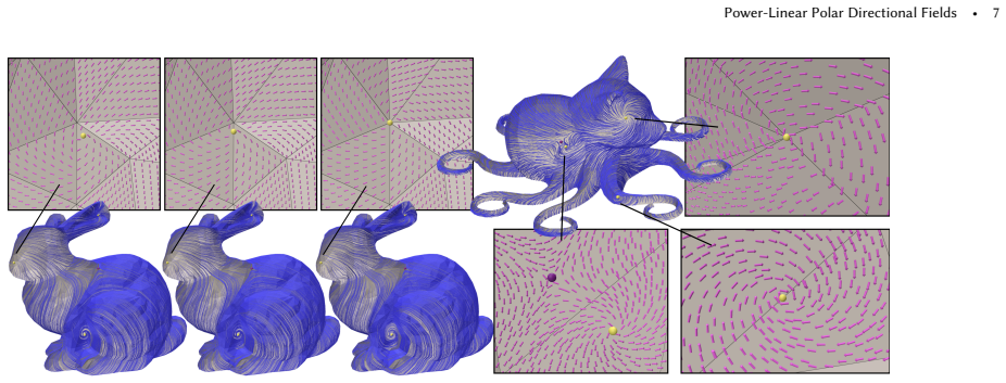
Coarse or uneven triangulations produce smoother fields than piecewise-constant polar methods, which the paper demonstrates on meshes of varying triangle quality.
Feature alignment along prescribed curves can be added by constraining half-cycles and a synchronization phase, without altering the topological constraints.
Higher-index singularities no longer require dense refinement to resolve, since the power-linear interpolant carries the rotation inside each triangle.

Reading between the lines

Editorial extensions of the paper, not claims the author makes directly.

If the reconstruction step preserves what the optimization promises, this representation should make quad- and hex-meshing pipelines less sensitive to mesh quality, since singularity placement no longer needs to wait for vertex creation.
A natural testable extension is to couple the polar singularity prescription with a Cartesian energy such as a Ginzburg-Landau functional, letting an optimizer propose singularity sets that the power-linear representation then realizes exactly.
The paper's own discussion suggests quadratic fields are problematic for exact index reproduction; one could probe the boundary of this by checking whether any higher-than-linear polar space can keep the exactness property the authors claim for power-linear fields.
The scale-based parametrization of face singularity location could be used as an interactive design handle: dragging a singularity inside a face would correspond to adjusting corner scales, which the current pipeline already exposes as constraints.

Share X Bluesky LinkedIn Reddit HN

Editorial analysis

A structured set of objections, weighed in public.

Desk editor's note, referee report, and a circularity audit.

Desk Editor's Note

read the letter

Short version: this is a real advance in polar directional fields, and the problems are fixable. The paper gives the first higher-order polar representation — piecewise power-linear fields u(z) = (a z + b z-bar + c)^I — on a beveled mesh, letting you put singularities of arbitrary integer index on faces, edges, or vertices, with N-fold symmetry. That is new. The appendix derivations for the winding-number targets and scale constraints are mathematically sensible, and the beveled combinatorial structure is a genuinely useful trick for homogenizing the treatment of faces, edges, and vertices.

What it does well: the power-linear extension is a natural but non-obvious step beyond trivial connections and previous low-order polar methods. The treatment of higher genus and boundaries via added cycle constraints is careful. The figures look convincing, and the comparison to trivial connections shows a clear qualitative improvement on coarse and uneven meshes.

Now the soft spots, in proportion. First, two equations in the main text are printed wrong. Eq. 5 is sigma_i sigma_j - sigma_j sigma_i = 0, which is an identity, so the face-scale constraint is vacuous as written; the real constraint lives in Appendix A.3. Eq. 10 has (theta_S - theta_S)^T ... which is identically zero, so the isotropy prior vanishes from the objective as printed. These are obvious typos, but they sit at the center of the method and need correcting before the main text can be trusted.

Second, the deeper issue: the optimization relaxes theta to piecewise constant and sigma to piecewise linear, and the final field is recovered by a separate linear solve in Global Integration. The paper does not show that this reconstruction preserves the optimized variables, the prescribed singularity locations, or the scale constraints. The authors' own note that the metric approximation 'favors more constant gradients and bigger jumps' concedes the objective is only a proxy. Without an experiment checking the actual singularity positions and the actual energy of the reconstructed field, the central claim — smooth fields with exact singularities anywhere — is not fully supported.

Third, no code or data, and the only baseline is trivial connections. That is thin for an applied geometry-processing paper.

None of this kills the core idea. The representation is new, the appendix mathematics looks right, and the gaps are addressable. A referee can ask for the typos fixed, the reconstruction verified numerically, and a broader comparison. I would send it out rather than desk-reject. The paper is honest about its limitations, which counts for something.

Referee Report

4 major / 4 minor

Summary. The paper introduces a polar (phase/scale) representation of directional fields on triangle meshes using piecewise power-linear interpolants. It proposes a beveled-mesh construction that turns all singularities, including those placed on faces, edges, or vertices, into face cycles in a single combinatorial structure, and formulates optimization problems for the phase 1-form and scale 0-form under cycle constraints. The power-linear extension and N-symmetric fields are presented as generalizations that support arbitrary integer indices and fractional N-fold symmetry indices. The paper reports results on meshes of varying quality and topology, with comparisons to trivial connections.

Significance. If the central claims are substantiated, this would be the first higher-order polar directional-field representation, with explicit user control over singularity location on any mesh element and support for arbitrary index and N-symmetry. The beveled-mesh construction is a clean conceptual contribution, and the appendix contains the substantive derivations (winding-number constraints, isotropic theta values, scale constraints from singularities, and the D-matrix construction). The paper does not ship code, but the algorithmic description is reasonably detailed. However, the main text as printed contains two vacuous formulas in the load-bearing constraint and objective, and the reconstruction step is not verified to preserve the prescribed singularities; these issues currently prevent the strongest claims from being considered established.

major comments (4)

[Sec. 4.1, Eq. (5)] The printed face-scale constraint sigma_i sigma_j - sigma_j sigma_i = 0 is an identity and imposes no restriction. Appendix A.3 shows that the intended condition is the complex equation u(s) = B_i sigma_i e^{i psi_i} + B_j sigma_j e^{i(psi_i+theta_ij)} + B_k sigma_k e^{i(psi_i+theta_ij+theta_jk)} = 0, which genuinely constrains the scale values so that the prescribed singularity position s is a zero of the interpolated field. Since the exact reproduction of face singularities rests on this constraint, the main text must state the correct equation (or an explicit equivalent ratio form), and the optimization system in Sec. 4.2 must be read with that correction.
[Sec. 4.2, Eq. (10)] The isotropy-attraction term as printed is lambda_S (theta_S - theta_S)^T D_S^T M_S D_S (theta_S - theta_S), which is identically zero. The intended term is evidently lambda_S (theta - theta_S)^T D_S^T M_S D_S (theta - theta_S). As written, the objective contains no attraction toward the prescribed isotropic theta_S values, so the claim that the field is as isotropic as possible in singular elements is not realized by the displayed system. The equation must be corrected and the implementation must be checked against the corrected term.
[Sec. 4.2, Global Integration; Sec. 5] The final field is recovered by a separate linear solve for corner values u, not by direct evaluation of the optimized theta and sigma. The paper does not prove that this reconstruction preserves the prescribed zero locations or the per-face indices, and the reported experiments do not verify this quantitatively: the comparison in Sec. 5 reports only the phase Dirichlet energy of theta, not the index or singularity-location error of the reconstructed field. The global-integration system is overdetermined as written, and no solution strategy (exact versus least squares) is specified, which further weakens the claim of exact singularity reproduction. The authors' own remark in Sec. 4.2 that the metric approximation favors more constant gradients and bigger jumps concedes that the optimized objective is a proxy; a quantitative check that the final field actually has the prescribed singularities at the prescribed locations is therefore needed.
[Sec. 4.4] The per-face index I_f is obtained by Dirichlet-energy interpolation followed by rounding to the nearest integer. This step is heuristic, and the paper gives no argument that rounding preserves the prescribed index balance or that a face whose I_f is rounded differently cannot introduce or remove a singularity. Since the central claim is control of arbitrary singularity indices, this step needs either a proof or an explicit numerical verification that the computed index of every face matches the prescribed value. In addition, the reconstruction formulas sigma_i^{1/I_f} and (B_i u_i + B_j u_j + B_k u_k)^{I_f} require branch specifications for negative I_f, which the paper does not provide.

minor comments (4)

[Sec. 4.1, Eqs. (6)-(7)] The part-edge variables theta_{sk,f}, theta_{ks,g}, and the orientation of the half-cycles are not fully defined in the main text; the inset and Sec. A.3.1 clarify them, but the main text should state the convention explicitly since Eq. (6) is used to justify later constraints.
[Sec. 4.2] The dimensions of the matrices D_S, M_S, and the construction of D_S from slices of D are only sketched in the main text; the appendix gives the D construction, but a short statement of the row grouping (which rows correspond to vertex flaps, edge flaps, and singular faces) would make the optimization systems self-contained.
[Sec. 5] The quantitative comparison reports only the phase Dirichlet energy of the edge-based theta. For a paper whose main claim is smoothness and exact singularity placement, it would be informative to also report energies or errors computed on the reconstructed field, such as the distance from the prescribed singularity location to the actual zero set, and the angle deviation of the field from the prescribed N-symmetry.
[Throughout] The manuscript contains several typographical issues that should be cleaned up: Eq. (5) and Eq. (10) as discussed above, the inconsistent use of M for the mesh and for the mass matrix, and the capital This in the middle of Sec. 3.3. None of these affect the underlying ideas, but they impede reading.

Circularity Check

1 steps flagged · score 6.0 of 10

Smoothness comparison is self-referential: the reported phase Dirichlet energy is the objective minimized in Eq. 10, so the claimed low-energy advantage is forced by construction; the representation itself is not circular.

fitted input called prediction [Section 5, 'Comparison to trivial connections'; Section 4.2, Eq. 10]
"θ = argmin [ θ^T D^T M_E D θ + λS(θS−θS)^T D^T_S M_S D_S(θS−θS) ], d1θ = 2πI−κ. ... For a quantitative comparison, we evaluate the phase Dirichlet energy E = θ^T L θ (Sec. 4.2), averaged by the number of faces, and where we upsample it uniformly to its three corners."

Equation 10 directly minimizes the quadratic form θ^T D^T M_E D θ as its smoothness objective, and Section 4.2 identifies θ as the differential quantity whose Dirichlet energy is built from D, M_E, and L. The Section 5 metric E = θ^T L θ is thus the same objective being optimized, not an independent measure of smoothness. The quantitative claim that the method produces smoother fields than Trivial Connections is therefore a restatement of the optimization target: the method's θ is fitted to minimize E, so reporting lower E is forced by construction rather than being an observed, external advantage. This is the fitted-input-called-prediction pattern in which the evaluation criterion is the same functional used to fit the field.

full rationale

The representation and singularity-placement machinery are not circular: power-linear fields are defined with prescribed indices, and the appendix gives explicit scale constraints for face and edge singularities; the cited X1 space from Boksebeld and Vaxman 2022 is acknowledged and is not the load-bearing argument. The one genuine circularity is the quantitative smoothness comparison, where the metric is the very quadratic form minimized in Eq. 10, so the reported advantage is a restatement of the objective. Separately, the main text contains two vacuous formulas: Eq. 5 is σ_i σ_j − σ_j σ_i = 0 and the isotropy term in Eq. 10 is (θS−θS), both identities, so the printed derivation of the singularity constraints does not perform the claimed work; the real constraints are deferred to Appendix A.3, and Section 4.2 admits the metric approximation is empirical. These are correctness and evidence gaps rather than circularity, but they mean the central 'anywhere on the mesh' claim is not established by the main-text equations as printed. Net score reflects the self-referential evaluation while recognizing that the core polar power-linear construction has independent content.

Assumptions & free parameters 4 free parameters · 6 assumptions · 1 invented entities

The central construction rests on hand-chosen parameters (lambda_S = 50, lambda_J = 50, epsilon = 1e-6), a new combinatorial beveled mesh, and several heuristic prescriptions (vertex isotropy, edge mid-phase, I_f rounding). The core representation and the winding-number constraints are derived from standard complex analysis, but the optimization and reconstruction involve modeling choices that are not derived from first principles.

free parameters (4)

lambda_S = 50
Isotropy penalty weight for singular elements, chosen by hand in Sec. 4.2 (Sys. 8, 10); no automatic selection or ablation is shown for this value.
lambda_J = 50
Jump penalty coefficient in the finite-volume energy, chosen by hand in Sec. 4.2; an ablation is shown in Fig. 9, but the choice remains manual.
epsilon = 1e-6
Lower bound for scale positivity (sigma >= epsilon), chosen by hand in Sec. 4.2 to keep scales from crossing zero.
middle phase selection at edge singularities (psi_sf) = (psi_1 + psi_2)/2
In appendix A.3.1, the phase at the edge singularity is set to the midpoint of the feasible interval; this ad hoc rule determines how the full edge theta is split into part-edge values.

assumptions (6)

standard math Index theorem: the sum of user-prescribed singularity indices must equal the Euler characteristic of the mesh (Sec. 4.1).
Used to make the prescribed singularity set realizable on a closed or bounded manifold triangle mesh.
standard math Winding-number formula (argument principle) for isotropic phase values: for a face singularity, theta_ij = I_f * angle subtended by edge ij at the singularity (Eq. 12 in appendix A.2).
This is the principal branch of the phase gradient of (z - s)^{I_f}; it is used to define the target theta for singular faces and edges.
ad hoc to paper The beveled-mesh construction (virtual edge-faces and vertex-faces, Sec. 4) renders all singularities as face cycles in a single structure, and the discrete cycle constraint d1 theta = 2 pi I - kappa (Eq. 4) is exact for this structure.
This is a new combinatorial model introduced by the paper; no formal proof is given that the beveled constraints are necessary and sufficient to reproduce a power-linear field with the prescribed topology.
ad hoc to paper Finite-volume relaxation: approximating theta as piecewise constant and sigma as piecewise linear, plus a jump penalty lambda_J, yields a faithful metric for field smoothness (Sec. 4.2).
The authors state this is an approximation and that it empirically favors constant gradients and larger jumps; the reconstruction step is not proven to attain the optimized energy.
domain assumption Vertex singularity isotropy prescription (appendix A.2, items 1-4): distributing rotation by flap angles approximates an ideal (z - v)^{I_v} field near the vertex when curvature is zero.
There is no unique ideal vertex field on a curved discrete surface; the prescription is a reasonable heuristic, not a derivation.
ad hoc to paper For power fields, the per-face index I_f is interpolated by minimizing Dirichlet energy and rounded to the nearest integer (Sec. 4.4).
Rounding can perturb the interpolated index field; the paper assumes this does not break the prescribed singularity topology.

invented entities (1)

Beveled mesh (virtual edge-faces and vertex-faces)
purpose: Adds a combinatorial face for each edge and vertex so that every singularity (face, edge, or vertex) becomes a face cycle in one uniform structure, simplifying the constraint system.
This is a new combinatorial construction (Sec. 4) with no falsifiable prediction outside the paper; its validity is judged only through the resulting fields. It is a structural device rather than a physical postulate.

how reviews work

0 comments

Cite this review

Pith. "Pith review of Power-Linear Polar Directional Fields." pith.science (2026). https://pith.science/paper/RFZ656IB

@misc{pith2026250600222,
  author       = {Pith},
  title        = {Pith review of: Power-Linear Polar Directional Fields},
  year         = {2026},
  howpublished = {\url{https://pith.science/paper/RFZ656IB}},
  note         = {Machine review of arXiv:2506.00222}
}

read the original abstract

We introduce a novel method for directional-field design on meshes, enabling users to specify singularities at any location on a mesh. Our method uses a piecewise power-linear representation for phase and scale, offering precise control over field topology. The resulting fields are smooth and accommodate any singularity index and field symmetry. With this representation, we mitigate the artifacts caused by coarse or uneven meshes. We showcase our approach on meshes with diverse topologies and triangle qualities.

Figures

Figures reproduced from arXiv: 2506.00222 by the authors.

**Figure 1.** We compute rotationally-smooth directional fields by prescribing their topology explicitly. Our fields (left) are piecewise power-linear, and therefore [PITH_FULL_IMAGE:figures/full_fig_p001_1.png] view at source ↗

**Figure 2.** (Left) An elliptic field with a +1 singularity, (middle) a linear singularity, and (right) a parabolic field with a −1 singularity. non-smooth for bad meshes (Figs. 1 and 14). We next show how to mitigate these effects using higher-order fields. 3.2 Representation We introduce piecewise-linear single-vector fields on simply-connected meshes, and generalize them to non-simply-connected meshes in Sec. 4.3 and power f… view at source ↗

**Figure 4.** There is a 2-dimensional space of fields with the same edge 𝜃, differing in the location of the singularity (red). We show three such examples. The integral in Eq. 2 is then discretized into 𝜃𝑖𝑗 + 𝜃 𝑗𝑘 + 𝜃𝑘𝑖 = 𝐼 𝑓 , the index of the triangle. For a linear field, this is the index of the only singularity that might be within the triangle (𝐼 𝑓 = 0 otherwise). The integrated edge-based 𝜃 representation is comfortable … view at source ↗

Figures from the paper (9 more)

**Figure 6.** Figure 6: Our linear field on simply-connected meshes. Our result is stable to small perturbations (left), and results in smooth fields for different indices (right). [PITH_FULL_IMAGE:figures/full_fig_p007_6.png]

**Figure 7.** Figure 7: A higher-genus example, where we vary the index [PITH_FULL_IMAGE:figures/full_fig_p007_7.png]

**Figure 11.** Figure 11: Higher-order singularities are well-captured by our method, on vertices, edges, or faces, due to our power-linear representation. [PITH_FULL_IMAGE:figures/full_fig_p009_11.png]

**Figure 12.** Figure 12: 𝑁 -fields with vertex, edge, and face singularities of different indices [PITH_FULL_IMAGE:figures/full_fig_p009_12.png]

**Figure 13.** Figure 13: Our method produces similar fields for the same geometry, despite considerable differences in mesh quality. [PITH_FULL_IMAGE:figures/full_fig_p009_13.png]

**Figure 14.** Figure 14: Comparison to trivial connections. It is apparent that our method, due to being of a higher order, accommodates higher-order singularities and uneven [PITH_FULL_IMAGE:figures/full_fig_p010_14.png]

**Figure 15.** Figure 15: Notation for vertex singularity 𝜃 isotropy prescription [PITH_FULL_IMAGE:figures/full_fig_p011_15.png]

**Figure 16.** Figure 16: Notation for edge singularity 𝜃 isotropy prescription. to which the corner field values are: 𝑢𝑖 = 𝜎 𝑖 𝑒 𝑖𝜓𝑖 , 𝑢𝑗 = 𝜎 𝑗 𝑒 𝑖(𝜓𝑖+𝜃𝑖 𝑗 ) , 𝑢𝑘 = 𝜎 𝑘 𝑒 𝑖(𝜓𝑖+𝜃𝑖 𝑗 +𝜃𝑗𝑘 ) , and where 𝑠 = 𝐵𝑖𝑧𝑖 + 𝐵𝑗𝑧𝑗 + 𝐵𝑘 𝑧𝑘 , for barycentric coordinates 𝐵𝑖,𝑗,𝑘 . We then have the linear relati…

**Figure 17.** Figure 17: Discrete segments of an alignment curve. [PITH_FULL_IMAGE:figures/full_fig_p012_17.png]

Discussion (0). Sign in to comment.

Reference graph

Works this paper leans on

2 extracted references

[2019]

ACM Trans

Weaving geodesic foliations. ACM Trans. Graph. 38, 4, Article 34 (July 2019), 22 pages. doi:10.1145/3306346.3323043 Floor Verhoeven, Amir Vaxman, Tim Hoffmann, and Olga Sorkine-Hornung. 2022. Dev2PQ: Planar Quadrilateral Strip Remeshing of Developable Surfaces. ACM Transactions on Graphics (TOG) (2022). Ryan Viertel and Braxton Osting. 2019. An Approach t...

arXiv 2022
[2022]

ACM Trans

Covector fluids. ACM Trans. Graph. 41, 4, Article 113 (July 2022), 16 pages. doi:10.1145/3528223.3530120 Jonathan Palacios and Eugene Zhang. 2007. Rotational Symmetry Field Design on Surfaces. ACM Transactions on Graphics 26, 3 (2007). David Palmer, Albert Chern, and Justin Solomon. 2024. Lifting Directional Fields to Minimal Sections. ACM Trans. Graph. 4...

arXiv 2007

Pith tools

Reviewed August 7, 2026 · model on record in the stance chip above.

[1] [2019]

ACM Trans

Weaving geodesic foliations. ACM Trans. Graph. 38, 4, Article 34 (July 2019), 22 pages. doi:10.1145/3306346.3323043 Floor Verhoeven, Amir Vaxman, Tim Hoffmann, and Olga Sorkine-Hornung. 2022. Dev2PQ: Planar Quadrilateral Strip Remeshing of Developable Surfaces. ACM Transactions on Graphics (TOG) (2022). Ryan Viertel and Braxton Osting. 2019. An Approach t...

arXiv 2022

[2] [2022]

ACM Trans

Covector fluids. ACM Trans. Graph. 41, 4, Article 113 (July 2022), 16 pages. doi:10.1145/3528223.3530120 Jonathan Palacios and Eugene Zhang. 2007. Rotational Symmetry Field Design on Surfaces. ACM Transactions on Graphics 26, 3 (2007). David Palmer, Albert Chern, and Justin Solomon. 2024. Lifting Directional Fields to Minimal Sections. ACM Trans. Graph. 4...

arXiv 2007