REVIEW 4 major objections 4 minor 49 references
Blind Sparse Estimation of Intermittent Sources over Unknown Fading Channels
T0 review · 4 major / 4 minor · reviewed 2026-08-14 · deepseek-v4-flash
Pith's one-line read A two-stage algorithm—smooth dictionary learning followed by per-source stochastic filtering—separates intermittent radio sources from fewer sensors over unknown flat-fading channels.
desk verdict A useful practical combination of smooth dictionary learning and per-source HMM post-filtering for intermittent sources, with a load-bearing ADMM derivation that needs fixing and a BAC model that deserves validation. read the letter →
The pith
A machine-rendered reading of the paper's core claim, the machinery that carries it, and where it could break.
The reading
What carries the argument
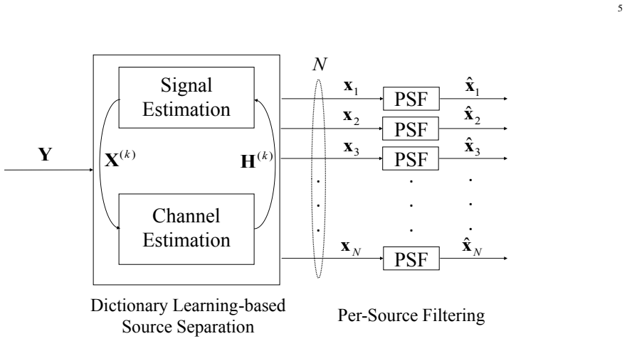
The load-bearing mechanism is the pairing of a smoothness prior with a noise model on activity estimates. Smooth LASSO adds the penalty term μ Σ_t ||x(t) − x(t−1)||_2 to the dictionary-learning signal update, encoding the prior that bursts last many samples, with SL-SEQ and SL-ADMM as low-complexity approximations. The per-source stochastic filtering stage then quantizes each source's estimated signal into a binary activity sequence and models that sequence as the output of a binary asymmetric channel with flip probabilities p'_n and q'_n, so the forward-backward algorithm can compute MAP activity states; EM updates both HMM transition probabilities and flip probabilities from the data. The binary-asymmetric-channel model is what converts dictionary-learning mistakes into a tractable filtering problem.
What would settle it
Generate the same N=30, M=20, T=1000 scenario but replace the independent binary-asymmetric-channel flips in the PSF model with a Markov chain of flips, or with flip probabilities that depend on the transmitted symbol, then run the proposed algorithm and check whether the detection probability at 0.1 false-alarm probability and 30 dB SNR remains near 0.96; a drop toward the no-PSF level would confirm that the memoryless-BAC premise is carrying the result.
Extended reading notes
Core claim
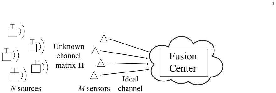
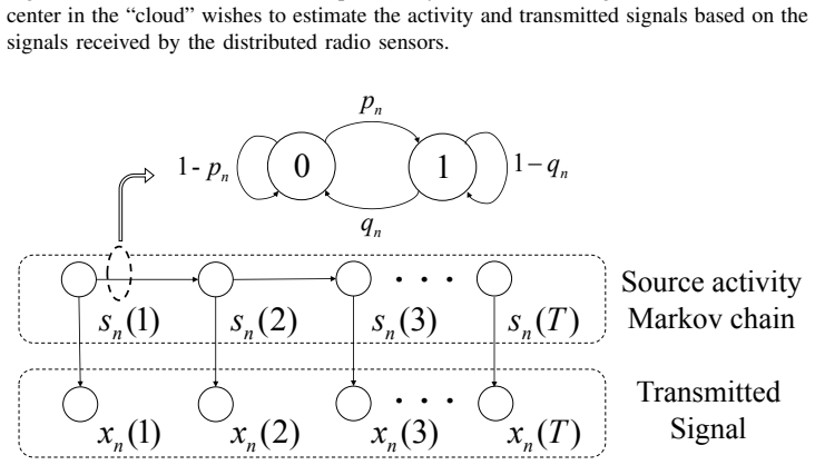
The paper claims that in the model Y = HX + Z with more sources than sensors, X column-sparse with hidden-Markov-driven on/off states and H constant over the observation window, the fusion center can estimate H, X, and the activity states blindly by alternating channel and signal updates, with the signal step using smooth LASSO to penalize short transmissions, followed by a per-source filtering stage. The filtering stage thresholds each source's estimated signal into a binary activity sequence, models that sequence as the output of a binary asymmetric channel with flip probabilities, and runs forward-backward MAP estimation, with EM estimating both the HMM transition probabilities and the flip probabilities when they are unknown. In simulation with 30 potential sources, 20 sensors, an average of 3 active sources per time sample, 1000 time samples, and 30 dB SNR, per-source filtering raises the probability of detection from 0.9 to 0.96 at 0.1 false-alarm probability and reduces the error vector magnitude by about 40 percent; with EM-estimated parameters the gain remains, though somewhat reduced.
Load-bearing premise
The whole per-source filtering gain rests on the assumption in Sec. V-A that the dictionary-learning stage's activity mistakes are independent, per-time flips with fixed probabilities; the paper does not justify this memoryless binary-asymmetric-channel model, so if the mistakes are correlated over time or across sources, the reported detection gain is not guaranteed.
Editorial extensions
If this is right
- In IoT-style settings with bursty transmitters, a fusion center can monitor more sources than antennas and still detect which are active, provided the activity patterns have memory and the channel is roughly constant over the observation block.
- The smooth-LASSO front end alone already outperforms memory-agnostic OMP and LASSO baselines in the paper's simulations, and per-source filtering adds a further gain on top.
- When HMM transition probabilities are unknown, EM-based per-source filtering recovers most of the detection gain, so the method does not require prior knowledge of burst statistics.
- The reported gain is robust to the sparsity level for the smooth-LASSO plus filtering scheme, while the baseline schemes degrade sharply as the average number of active sources increases.
Reading between the lines
- An unstated corollary is that the method's success depends on bursts being long relative to the dictionary-learning window; if transmission durations shrink toward single symbols, the smoothness penalty has nothing to exploit and the per-source filter loses its edge.
- If the binary-asymmetric-channel independence assumption fails, for instance when a missed detection makes nearby misses more likely, a natural extension is to model the flip process itself as Markov or to filter all sources jointly, which could preserve the gain in correlated-error regimes.
- Because the two stages communicate only one-way, feeding the cleaned activity states back into the dictionary-learning objective as a warm start could further sharpen channel and signal estimates; the paper does not explore this closed-loop variant.
Signed reviews
Editorial analysis
A structured set of objections, weighed in public.
Referee Report
Summary. The paper considers blind estimation of N sparse, intermittently active sources from M<N sensors over unknown slow flat-fading channels, with source activity modeled as a two-state HMM. It proposes a two-stage algorithm: a dictionary learning stage with a smooth LASSO penalty on temporal activity changes (implemented as SL-SEQ and SL-ADMM), followed by per-source stochastic filtering that thresholds the DL activity estimates and passes them through a forward-backward HMM filter (with EM when HMM/BAC parameters are unknown). Numerical experiments with N=30, M=20, T=1000 report that the proposed SL+PSF method outperforms OMP and LASSO baselines in detection and EVM, including robustness to sparsity.
Significance. If validated, the architecture is a sensible combination of sparse dictionary learning and HMM-based post-filtering that addresses an underdetermined, bursty-source scenario of practical IoT interest. The paper's reported gains—e.g., Pd from 0.9 to 0.96 at Pfa=0.1 with unknown parameters, and a 40% EVM reduction—are nontrivial. The simulation study is fairly extensive, covering ROC curves, SNR, sparsity level, known/unknown parameters, and multiple baselines; the two-stage idea is clearly presented. However, the support is empirical and rests on several model assumptions that need to be checked before the central claim is fully established.
major comments (4)
- [Sec. IV-B, Eqs. (9)-(12)] There is a mismatch between the constraint and the dual update in the SL-ADMM derivation. Problem (9) imposes x'(t)=x(t) for t=1,...,T-1 and the augmented Lagrangian in (10) contains alpha^T(t)(x(t)-x'(t)), but the dual update in (12) uses x'(i)(t-1) rather than x'(i)(t). Moreover, (10) adds a rho-term on ||x(t)-x'(t-1)||2 while the constraint is on x(t)-x'(t); this corresponds to a different consensus problem. The text should correct the formulation and confirm that the implemented algorithm actually solves (7), or derive the correct ADMM updates.
- [Sec. V-A, Eq. (13)] With alpha_t defined as the filtered posterior Pr(s_n(t)=1|s_tilde(1:t)) and beta_t as the backward likelihood Pr(s_tilde(t+1:T)|s_n(t)=1), the equality Pr(s_n(t)=1|s_tilde(1:T)) = alpha_t beta_t is not correct; the right side is not normalized and can exceed one. The standard forward-backward posterior requires alpha_t to be the joint forward variable, or the final product must be normalized by the total observation likelihood. Please correct the definition or equation and ensure the MAP threshold comparison uses a proper probability.
- [Sec. V-A, Fig. 4 and Sec. VI] The PSF gain in the Conclusions depends on modeling the thresholded DL activity estimates as outputs of a memoryless binary asymmetric channel with fixed flip probabilities p'_n=0.02 and q'_n=0.27. The paper does not validate that the DL error process is memoryless, time-independent, or source-independent; errors produced by iterative dictionary learning are functions of the entire burst and the learned dictionary and can be correlated. Please add an empirical analysis of the activity-error process (e.g., autocorrelation of s_tilde_n(t)-s_n(t) and pairwise cross-correlation across sources), and report sensitivity of the Pd/Pfa curves to p' and q' or to using EM-estimated values instead of fixed ones.
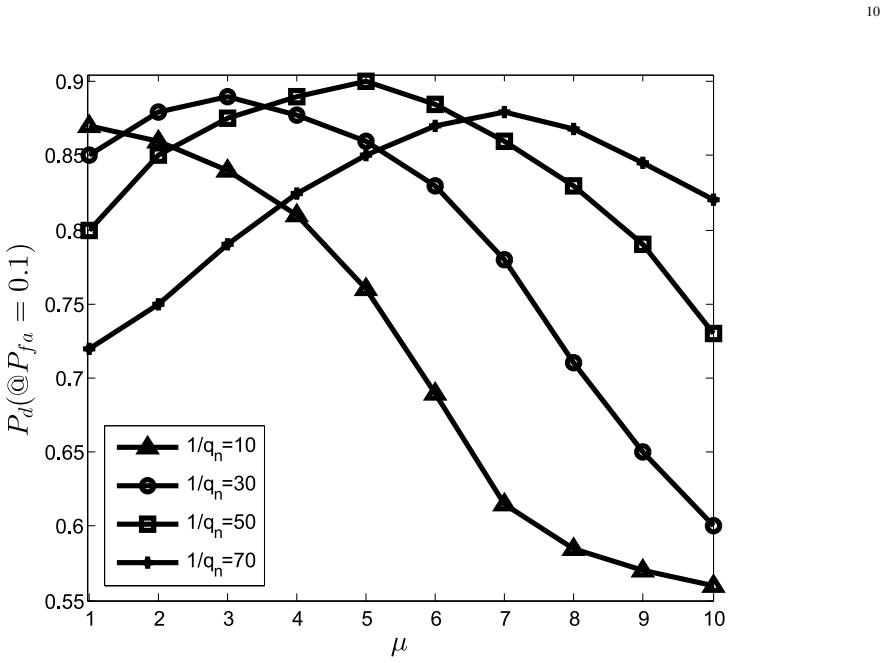
- [Sec. VI-A] The statement that lambda and mu are optimized to satisfy given constants on Pd or Pfa is ambiguous: if this optimization uses the true activity labels, the reported ROC curves depend on oracle tuning, and it is unclear whether the OMP and LASSO baselines receive equally favorable tuning. Please specify the tuning protocol (grid, criterion, ground-truth dependence) and apply the same protocol to all compared algorithms.
minor comments (4)
- [Sec. II] Near the top of Sec. II, 'the fusion center has access to N receive antennas' should read 'M receive antennas', since the model uses M sensors.
- [Sec. II] The definition of the transition probabilities has a subscript typo: p_n = Pr(s_n(t)=1|s_{n-1}(t)=0) should be Pr(s_n(t)=1|s_n(t-1)=0), and similarly for q_n.
- [Sec. V-A] The MAP decision uses the same symbol s_hat_n(t) for both the quantized DL activity estimate and the final MAP estimate; using distinct notation would avoid confusion.
- [Sec. VI-C and Sec. VII] The EVM results condition on the set of correctly detected active time samples, which can favor methods with conservative detection; this conditioning should be stated more prominently. Also, the Conclusion contains a typo, 'decrease the EVM from by 40%'.
Circularity Check
No significant circularity: the PSF detection gain is a simulation result measured against ground-truth activity and independent baselines, not a quantity constructed from the algorithm's own fitted outputs.
full rationale
The paper's derivation chain is self-contained and contains no step in which a 'prediction' reduces by construction to a fitted input or to a self-citation. The DL stage solves a smooth-LASSO problem (Eq. (7)) whose parameters lambda and mu are tuned numerically, and the PSF stage assumes a memoryless binary asymmetric channel for the quantized DL activity estimates (Fig. 4 and Eq. (13)). The BAC flip probabilities are either fixed simulation parameters (p' = 0.02, q' = 0.27) or estimated from the DL output via EM (Eqs. (17)-(18)); they are not fitted to the ground-truth detection probability that the paper claims to improve. The reported gain from 0.9 to 0.96 detection probability is obtained by comparing SL-ADMM with and without PSF on synthetic data generated from a known HMM, where the baselines OMP and LASSO are independent of the PSF model. No uniqueness theorem is imported from the authors' prior work, and the cited references are external standard methods. The main weakness, namely that the BAC assumption is not validated against temporally correlated DL errors, is a model-misspecification or robustness concern, not a circularity: the paper does not define the detection improvement in terms of the BAC posterior it assumes. Thus the appropriate finding is no significant circularity.
Assumptions & free parameters
free parameters (7)
- lambda (sparsity penalty) =
lambda = 1/SNR (rule of thumb, numerically tuned)
- mu (temporal smoothness penalty) =
mu = 0.1/q_n, with q_n the true transition probability
- gamma (state quantization threshold) =
0.5
- rho (ADMM penalty parameter) =
0.1
- K (SL-ADMM iterations) =
30
- BAC flip probabilities in known-parameter PSF =
p'_n = 0.02, q'_n = 0.27
- EM initialization and stopping tolerance =
p_n = 0.5, q_n = 0.5, p'_n = 0.1, q'_n = 0.2; epsilon unspecified
assumptions (5)
- domain assumption The channel H is constant over T symbol periods, noise is iid zero-mean complex Gaussian, sensors are time-synchronized, and backhaul to the fusion center is ideal.
- domain assumption Each source's activity s_n(t) follows a two-state Markov chain with transition probabilities p_n and q_n, and active transmissions are iid from a known distribution such as Gaussian or binary.
- domain assumption The alternating dictionary-learning minimization over (H, X) converges to a useful dictionary and sparse coefficient matrix despite being nonconvex and underdetermined.
- ad hoc to paper The quantized DL state estimates are related to the true states through a memoryless binary asymmetric channel with flip probabilities p'_n and q'_n.
- standard math Standard algorithms (forward-backward, EM, ADMM) converge to the claimed estimates in this setting.
invented entities (1)
-
Memoryless binary asymmetric channel (BAC) representing DL state errors
Cite this review
Pith. "Pith review of Blind Sparse Estimation of Intermittent Sources over Unknown Fading Channels." pith.science (2026). https://pith.science/paper/RK6BZ4IP
@misc{pith2026190801822,
  author       = {Pith},
  title        = {Pith review of: Blind Sparse Estimation of Intermittent Sources over Unknown Fading Channels},
  year         = {2026},
  howpublished = {\url{https://pith.science/paper/RK6BZ4IP}},
  note         = {Machine review of arXiv:1908.01822}
}
read the original abstract
Radio frequency sources are observed at a fusion center via sensor measurements made over slow flat-fading channels. The number of sources may be larger than the number of sensors, but their activity is sparse and intermittent with bursty transmission patterns. To account for this, sources are modeled as hidden Markov models with known or unknown parameters. The problem of blind source estimation in the absence of channel state information is tackled via a novel algorithm, consisting of a dictionary learning (DL) stage and a per-source stochastic filtering (PSF) stage. The two stages work in tandem, with the latter operating on the output produced by the former. Both stages are designed so as to account for the sparsity and memory of the sources. To this end, smooth LASSO is integrated with DL, while the forward-backward algorithm and Expectation Maximization (EM) algorithm are leveraged for PSF. It is shown that the proposed algorithm can enhance the detection and the estimation performance of the sources, and that it is robust to the sparsity level.
Figures
Figures from the paper (9 more)




Reference graph
Works this paper leans on
-
[1]
P. Comon and C. Jutten, Handbook of Blind Source Separation: Independent Component analysis and Applications . Cambridge: Academic press, 2010
work page 2010
-
[2]
S. Araki, R. Mukai, S. Makino, T. Nishikawa, and H. Saruwatari, “The fundamental limitation of frequency domain blind source separation for convolutive mixtures of speech,” IEEE Transaction on Speech and Audio Processing , vol. 11, pp. 109–116, 2003
work page 2003
-
[3]
Blind separation and dereverberation of speech mixtures by joint optimization,
T. Yoshioka, T. Nakatani, M. Miyoshi, and H. G. Okuno, “Blind separation and dereverberation of speech mixtures by joint optimization,” IEEE Trans. on Audio, Speech, and Language Processing , vol. 19, pp. 69–84, 2011. 13 Fig. 11: Estimation performance of p′ n and q′ n for BAC in the EM algorithm ( N = 30, M = 20, T = 1000, SNR= 30 dB, pn = 0.0022, qn = 0...
work page 2011
-
[4]
A. Cichocki and S.-i. Amari, Adaptive blind signal and image processing: learning algorithms and applications. Hoboken, NJ: John Wiley & Sons, 2002
work page 2002
-
[5]
Applications of neural blind separation to signal and image processing,
J. Karhunen, A. Hyv ¨arinen, R. Vigario, J. Hurri, and E. Oja, “Applications of neural blind separation to signal and image processing,” Acoustics, Speech, and Signal Processing, 1997. ICASSP-97., 1997 IEEE International Coference on , vol. 5, pp. 131–134, 1997
work page 1997
-
[6]
Blind separation of disjoint orthogonal signals: demixing N sources from 2 mixtures,
A. Jourjine, S. Rickard, and ¨O. Yilmaz, “Blind separation of disjoint orthogonal signals: demixing N sources from 2 mixtures,”Acoustics, Speech, and Signal Processing, 2000. ICASSP ’00. Proceedings. 2000 IEEE International Conference on, 2000
work page 2000
-
[7]
S. Wehr, I. Kozintsev, R. Lienhart, and W. Kellermann, “Synchronization of acoustic sensors for distributed ad-hoc audio networks and its use for blind source separation,” Multimedia Software Engineering, 2004. Proceddings. IEEE Sixth International Symposium on , 2004
work page 2004
-
[8]
Independent component analysis: algorithms and applications,
A. Hyv ¨arinen and E. Oja, “Independent component analysis: algorithms and applications,” Neural Networks, vol. 13, pp. 411–430, 2000
work page 2000
Show all 49 references
-
[9]
Principal component analysis,
S. Wold, K. Esbensen, and P. Geladi, “Principal component analysis,” Chemometrics and Intelligent Laboratory Systems , vol. 2, pp. 37–52, 1987
1987
-
[10]
Singular value decomposition and least squares solutions,
G. H. Golub and C. H. Reinsch, “Singular value decomposition and least squares solutions,” Numerische Mathematik , vol. 14, pp. 403–420, 1970
1970
-
[11]
Long-range communications in unlicensed bands: the rising stars in the IoT and smart city scenarios,
M. Centenaro, L. Vangelista, A. Zanella, and M. Zorzi, “Long-range communications in unlicensed bands: the rising stars in the IoT and smart city scenarios,” IEEE Wireless Communications, vol. 23, pp. 60–67, 2016
2016
-
[12]
New 3GPP standard for IoT,
J. Gozalvez, “New 3GPP standard for IoT,” IEEE Vehicular Technology Magazine, vol. 11, pp. 14–20, 2016
2016
-
[13]
Distributed linear blind source separation over wireless sensor networks with arbitrary connectivity patterns,
S. M. Alavi and W. B. Kleijn, “Distributed linear blind source separation over wireless sensor networks with arbitrary connectivity patterns,” Acoustics, Speech and Signal Processing, IEEE Transactions on , pp. 3171–3175, March 2016
2016
-
[14]
A blind source separation technique for spectrum sensing in cognitive radio networks based on kurtosis metric,
S. S. Ivrigh, S. M.-S. Sadough, and A. A. Ghorashi, “A blind source separation technique for spectrum sensing in cognitive radio networks based on kurtosis metric,” Computer and Knowledge Engineering (ICCKE), 2011 1st International eConference on, Oct. 2011
2011
-
[15]
Independent component analysis for semi-blind signal separation in MIMO mobile frequency selective communication channels,
D. Obradovic, N. Madhu, A. Szabo, and C. S. Wong, “Independent component analysis for semi-blind signal separation in MIMO mobile frequency selective communication channels,” Neural Networks, 2004. Proceedings. 2004 IEEE International Joint Conference on , July 2004
2004
-
[16]
Blind signal separation in MIMO OFDM system using ICA and fractional sampling,
S. R. Curnew and J. Ilow, “Blind signal separation in MIMO OFDM system using ICA and fractional sampling,” Signals, Systems and Electronics, 2007. ISSSE ’07. International Symposium on , Aug. 2007
2007
-
[17]
Hyv ¨arinen, J
A. Hyv ¨arinen, J. Karhunen, and E. Oja, Independent Component Analysis , 3rd ed. West Sussex, United Kingdom: John Wiley & Sons, 2004
2004
-
[18]
Elad, Sparse and Redundant Representations: From Theory to Applications in Signal and Image Processing
M. Elad, Sparse and Redundant Representations: From Theory to Applications in Signal and Image Processing . New York: Springer, 2010
2010
-
[19]
Sparse signal reconstruction from limited data using FOCUSS: a re-weighted minimum norm algorithm,
I. F. Gorodnitsky and B. D. Rao, “Sparse signal reconstruction from limited data using FOCUSS: a re-weighted minimum norm algorithm,” International Journal of Pattern Recognition and Artificial Intelligence , vol. 45, pp. 600–616, 1997
1997
-
[20]
Optimized orthogonal matching pursuit approach,
L. Rebollo-Neira and D. Lowe, “Optimized orthogonal matching pursuit approach,” IEEE Signal Processing Letters , vol. 9, pp. 137–140, 2002
2002
-
[21]
Dictionaries for sparse representation modeling,
R. Rubinstein, A. M. Bruckstein, and M. Elad, “Dictionaries for sparse representation modeling,” Proceedings of the IEEE, vol. 98, pp. 1045–1057, 2010
2010
-
[22]
Dictionary learning,
I. Tosic and P. Frossard, “Dictionary learning,” IEEE Signal Processing Magazine , vol. 28, pp. 27–38, 2011
2011
-
[23]
Joint DOA Estimation and Array Calibration Using Multiple Parametric Dictionary Learning,
H. Ghanbari, H. Zayyani, and E. Yazdian, “Joint DOA Estimation and Array Calibration Using Multiple Parametric Dictionary Learning,” ArXiv e-prints, Jul. 2017
2017
-
[24]
A Stochastic Successive Minimization Method for Nonsmooth Nonconvex Optimization with Applications to Transceiver Design in Wireless Communication Networks,
M. Razaviyayn, M. Sanjabi, and Z.-Q. Luo, “A Stochastic Successive Minimization Method for Nonsmooth Nonconvex Optimization with Applications to Transceiver Design in Wireless Communication Networks,” ArXiv e-prints, Jul. 2013
2013
-
[25]
Cloud K-SVD: A collaborative dictionary learning algorithm for big, distributed data,
H. Raja and W. U. Bajwa, “Cloud K-SVD: A collaborative dictionary learning algorithm for big, distributed data,” IEEE Transcations on Signal Processing , vol. 64, pp. 173–188, 2015
2015
-
[26]
Dictionary Learning Based Sparse Channel Representation and Estimation for FDD Massive MIMO Systems,
Y . Ding and B. D. Rao, “Dictionary Learning Based Sparse Channel Representation and Estimation for FDD Massive MIMO Systems,” ArXiv e-prints, Dec. 2016
2016
-
[27]
Independent vector analysis incorporating active and inactive states,
A. Masnadi-Shirazi and B. Rao, “Independent vector analysis incorporating active and inactive states,” Acoustics, Speech and Signal Processing, 2009. ICASSP 2009. IEEE International Conference on , May 2009
2009
-
[28]
Glimpsing independent vector analysis: Separating more sources than sensors using active and inactive states,
A. Masnadi-Shirazi, W. Wang, and B. Rao, “Glimpsing independent vector analysis: Separating more sources than sensors using active and inactive states,” Acoustics, Speech and Signal Processing (ICASSP), 2010 IEEE International Conference on, June 2010
2010
-
[29]
Synchronization for lassical blind source separation algorithms in wireless acoustic sensor networks,
C. Llerena, R. Gil-Pita, D. Ayllon, H. Sanchez-Hevia, I. Mohino-Herranz, and M. Rosa, “Synchronization for lassical blind source separation algorithms in wireless acoustic sensor networks,” 2016 IEEE Statistical Signal Processing Workshop (SSP), June 2016
2016
-
[30]
Blind synchronization in wireless acoustic sensor networks,
D. Cherkassky and S. Gannot, “Blind synchronization in wireless acoustic sensor networks,” IEEE/ACM Trans. on Audio, 15 Speech, and Language Processing , vol. 25, pp. 651–661, 2017
2017
-
[31]
Dictionary learning over distributed models,
J. Chen, Z. J. Towfic, and A. H. Sayed, “Dictionary learning over distributed models,” IEEE Trans. on Signal Processing, vol. 63, pp. 1001–1016, 2015
2015
-
[32]
Dictionary identification - sparse matrix-factorization via 𝓁1-minimization,
R. Gribonval and K. Schnass, “Dictionary identification - sparse matrix-factorization via 𝓁1-minimization,” IEEE Trans. on Information Theory , vol. 56, pp. 3523–3539, 2010
2010
-
[33]
Method of optimal directions for frame design,
K. Engan, S. O. Aase, and J. Hakon Husoy, “Method of optimal directions for frame design,” Proc, IEEE ICASSP, vol. 5, pp. 2443–2446, 1999
1999
-
[34]
Improving dictionary learning: Multiple dictionary updates and coefficient reuse,
L. N. Smith and M. Elad, “Improving dictionary learning: Multiple dictionary updates and coefficient reuse,” IEEE Signal Process. Lett., vol. 20, no. 1, pp. 79–82, 2013
2013
-
[35]
Dictionary training for sparse representation as generalization of k-means clustering,
S. K. Sahoo and A. Makur, “Dictionary training for sparse representation as generalization of k-means clustering,” IEEE Signal Process. Lett. , vol. 20, no. 6, pp. 587–590, 2013
2013
-
[36]
Dictionary learning for sparse representation: A novel approach,
M. Sadeghi, M. Babaie-Zadeh, and C. Jutten, “Dictionary learning for sparse representation: A novel approach,” IEEE Signal Process. Lett. , vol. 20, no. 12, pp. 1195–1198, 2013
2013
-
[37]
Regression shrinkage and selection via the lasso,
R. Tibshirani, “Regression shrinkage and selection via the lasso,” Journal of the Royal Statistical Society , vol. 58, no. 1, pp. 267–288, 1996
1996
-
[38]
Convolutional dictionary learning,
C. Garcia-Cardona and B. Wohlberg, “Convolutional dictionary learning,” CoRR, vol. abs/1709.02893, 2017. [Online]. Available: http://arxiv.org/abs/1709.02893
2017 arXiv
-
[39]
The smooth-lasso and other 𝓁1 +𝓁2-penalized methods,
M. Hebiri and S. van de Geer, “The smooth-lasso and other 𝓁1 +𝓁2-penalized methods,” Electronic Journal of Statistics , vol. 5, pp. 1184–1226, 2011
2011
-
[40]
An interior-point method for large-scale 𝓁1-regularized logistic regression,
K. Koh, S. J. Kim, and S. Boyd, “An interior-point method for large-scale 𝓁1-regularized logistic regression,” Journal of Machine Learning Research , vol. 8, pp. 1519–1555, 2007
2007
-
[41]
Regularization and variable selection via the elastic net,
H. Zou and T. Hastie, “Regularization and variable selection via the elastic net,” Journal of the Royal Statistical Society , vol. 67, pp. 301–320, 2005
2005
-
[42]
Distributed optimization and statistical learning via the alternating direction method of multipliers,
S. Boyd, N. Parikh, E. Chu, B. Peleato, and J. Eckstein, “Distributed optimization and statistical learning via the alternating direction method of multipliers,” Foundations and Trends in Machine Learning , vol. 3, pp. 1–122, 2011
2011
-
[43]
Proximal algorithms,
N. Parikh and S. Boyd, “Proximal algorithms,” Foundations and Trends in Optimization , vol. 1, pp. 123–231, 2014
2014
-
[44]
Multiplier and gradient methods,
M. R.Hestenes, “Multiplier and gradient methods,” Journal of Optimization Theory and Applications , vol. 4, pp. 302–320, 1969
1969
-
[45]
Koller and N
D. Koller and N. Friedman, Probabilistic Graphical Models: Principles and Techniques . Cambridge, Massachusetts: MIT Press, 2009
2009
-
[46]
K. P. Murphy, Machine Learning: A Probabilistic Perspective . Cambridge, Massachusetts: MIT Press, 2012
2012
-
[47]
C. M. Bishop, Pattern Recognition and Machine Learning . New York, NY: Springer, 2006
2006
-
[48]
An introduction to hidden markov models and bayesian networks,
Z. Ghahramani, “An introduction to hidden markov models and bayesian networks,” International Journal of Pattern Recognition and Artificial Intelligence , vol. 15, pp. 9–42, 2001
2001
-
[49]
Generalized elastic net regression,
G. Mouret, J.-J. Brault, and V . Partovinia, “Generalized elastic net regression,” the Joint Statistical Meetings , Aug. 2017
2017
Reviewed August 14, 2026 · model on record in the stance chip above.
Discussion (0). Continue with ORCID to comment.