REVIEW 4 major objections 7 minor 38 references
Bayesian Gaussian Mixture Modeling for Symmetric Matrix Variate Data
T0 review · 4 major / 7 minor · reviewed 2026-08-10 · deepseek-v4-flash
Pith's one-line read Mixture model reveals crime and youth jobs drive mobility overlap
desk verdict A genuinely useful reduced-order parameterization for symmetric matrix-variate precision matrices, but the m-selection evidence is thinner than the application's universal m=1 claim suggests. read the letter →
The pith
A machine-rendered reading of the paper's core claim, the machinery that carries it, and where it could break.
The reading
What carries the argument
The load-bearing object is the commutativity constraint $\Omega\Upsilon = \Upsilon\Omega$ in the symmetric matrix-variate normal distribution. Commutativity makes the two precision matrices simultaneously diagonalizable, so $\Upsilon$ can be expressed as a polynomial of $\Omega$; the model then restricts attention to a single active term $\Upsilon = aI + b\Omega^m$, with the polynomial order $m$ treated as an unknown parameter and selected by reversible-jump MCMC. The likelihood's normalizing constant is evaluated through the eigendecomposition of $\Omega$, avoiding explicit construction of the $p^2 \times p(p+1)/2$ transformation matrix $B_p$ and making the sampler computationally tractable.
What would settle it
Simulate 11 weekly sociomatrices from a symmetric matrix-variate normal mixture with non-commuting precision matrices and compare STRUCTURED-RJ's joint precision MSE to the unconstrained MVGGM; if the reduced model's MSE does not at least match the unconstrained model, the commuting assumption is doing the work.
Extended reading notes
Core claim
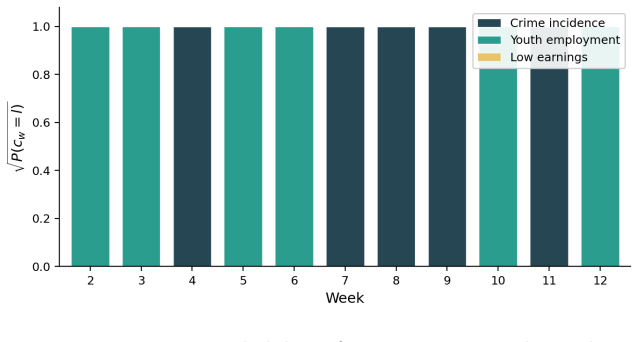
The central claim is that for symmetric matrix-variate normal data, commutativity of the row and column precision matrices forces the column precision to be a polynomial of the row precision, and that the reduced form $\Upsilon = aI + b\Omega^m$ with order $m$ chosen by reversible-jump MCMC captures that polynomial structure with three effective parameters. The paper argues that this reduction is what makes estimation feasible in sparse-data regimes, where an unconstrained estimator must fit $p(p+1)$ free elements per precision matrix. Simulation comparisons show STRUCTURED-RJ achieving roughly ten times lower joint-precision MSE than the unconstrained MVGGM when $\Upsilon = \Omega$, and outperforming all alternatives with as few as five observations per component. The application to GPS-derived sociomatrices of 293 King County residents identifies crime incidence and youth employment as the demographic similarity graphs that best explain weekly variation in activity overlap, with every component selecting $m=1$ and thus a shared conditional-independence graph for row and column precision.
Load-bearing premise
The model's conclusions stand only if the true row and column precision matrices commute and the column precision is exactly one active polynomial term; if either fails, the reduced parameterization is misspecified.
Editorial extensions
If this is right
- With as few as five observations per mixture component, the reduced-order parameterization delivers lower MSE than the unconstrained MVGGM, so short network time series become analyzable.
- Automatic selection of $m$ by reversible-jump MCMC costs almost nothing: STRUCTURED-RJ stays within about 5% of the oracle fixed-order model for $m=1$, so practitioners do not need to know the polynomial order in advance.
- For larger samples (about ten or more observations per component), the full-polynomial variant STRUCTURED-FP is the better choice, especially when the true relation has degree $m=2$.
- In the King County data, the same demographic similarity graph governs both row and column precision ($m=1$ for all components), which simplifies interpretation of activity-overlap networks.
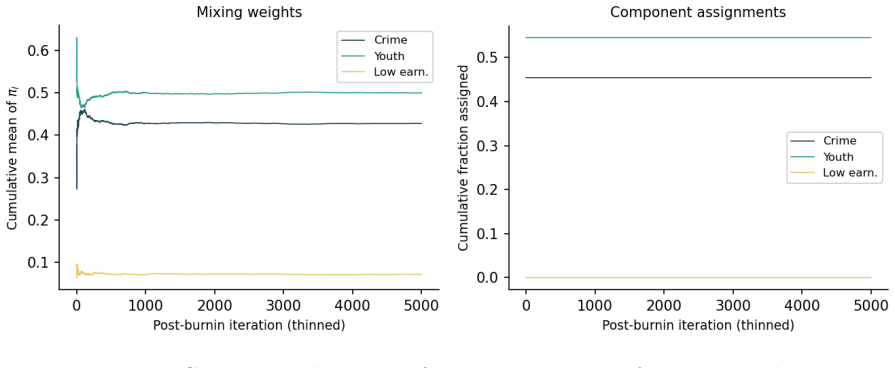
- The low-earnings employment graph is effectively inactive ($\hat{\pi}=0.07$), suggesting that local crime and youth employment density, not low-wage job density, are the demographic dimensions that differentiate weekly mobility overlap.
Reading between the lines
- If the commuting-precision assumption is plausible, the same parameter reduction transfers to other symmetric relational datasets with few temporal replicates, such as financial correlation networks or protein interaction snapshots.
- The reported crime/youth split depends on threshold-dichotomized demographic similarity graphs; replacing those thresholds with a fully Bayesian graph-selection prior would test whether the split is an artifact of the discretization.
- Adding temporal persistence across weeks, for instance a hidden Markov model on component labels, could reveal mobility regimes that last longer than a single week and sharpen the demographic interpretation.
Signed reviews
Editorial analysis
A structured set of objections, weighed in public.
Referee Report
Summary. The paper introduces STRUCTURED, a Bayesian mixture model for symmetric matrix-variate normal data. The key idea is to exploit the commutativity of the row and column precision matrices, Ω and Υ, to express Υ as a polynomial of Ω, and then to restrict the model to a single active polynomial term Υ = aI + bΩ^m, with the order m selected by reversible-jump MCMC (STRUCTURED-RJ) or a full polynomial (STRUCTURED-FP). Simulation studies claim that STRUCTURED-RJ outperforms the unconstrained MVGGM in sparse-data regimes, while STRUCTURED-FP is preferred for larger samples. The method is applied to weekly GPS-derived sociomatrices of individuals in King County, WA, where the mixture components are tied to demographic similarity graphs built from crime incidence and employment data, and the model assigns 5 weeks to crime and 6 weeks to youth employment, with m = 1 selected for all components.
Significance. If the theoretical and empirical claims were fully supported, the reduced parameterization for symmetric matrix-variate normal mixtures would be a useful contribution for high-dimensional sparse relational data. The paper is original in combining the symmetric matrix-variate normal distribution with a mixture over demographic graphs and in using reversible-jump MCMC to select the polynomial order. The application to GPS-derived activity overlap is timely and the comparison with MVGGM is a reasonable external baseline. However, several load-bearing points are not adequately established: the polynomial representation theorem is overstated, the reversible-jump procedure's ability to recover m = 2 is not demonstrated and the reported simulations suggest it may fail, and the application's m = 1 finding is likely dominated by the prior rather than the data. These gaps currently limit confidence in the central claim of accurate reduced-order estimation.
major comments (4)
- [Section 3, Theorem 3.1 and Appendix A.2] Theorem 3.1 claims that for any commuting Υ and Ω, Υ is a limit of polynomials in Ω + ε, even when Ω has repeated eigenvalues. This statement is not correct in general. For example, if Ω = I, then every polynomial in Ω + ε is scalar, so no limit of such polynomials can equal a non-scalar commuting Υ. The proof in Appendix A.2 approximates Ω by a simple-spectrum matrix but does not control the coefficients α_k(ε), and the limit need not be a polynomial in Ω. Since the polynomial parameterization is the methodological foundation, the authors should either restrict the theorem to the almost-sure case of simple eigenvalues and explicitly state the reduced form as a modeling assumption for the general case, or provide a correct proof.
- [Section 4, Tables 1 and 3] The paper never reports the posterior distribution of m for the simulation with true Υ = Ω^2. Table 1 reports P(m = 1) ≈ 0.84 for true m = 1, but for true m = 2 only MSEs are given. Table 3 shows that STRUCTURED-RJ's MSE for m = 2 is essentially flat (0.044, 0.045, 0.047, 0.052) as N increases from 5 to 50, whereas MVGGM improves from 0.145 to 0.029. If the sampler were correctly selecting m = 2, increasing N should reduce the RJ estimator's error; the flat profile instead suggests that the sampler frequently selects the prior-favored m = 1, imposing a misspecified linear structure. This is a load-bearing gap because the central claim that STRUCTURED-RJ accurately recovers the reduced-order parameterization depends on the sampler honestly identifying m.
- [Section 5, Table 4 and Figure 6] The application's universal posterior probability of 1.0 for m = 1 is not informative about the true polynomial order. With only N/L ≈ 4 effective observations per component and the geometric prior p(m) ∝ ρ^m, the prior will dominate the posterior, as the authors themselves note that the simulation advantage of STRUCTURED-RJ is confined to N ≤ 5 per component. The active components have 5 and 6 weeks, which is near the crossover where MVGGM and STRUCTURED-FP become competitive (Table 3), so the regime claim is fragile. The interpretation that 'Corr(Ω̂, Υ̂) = 1.00 confirms that the linear relationship Υ ≈ bΩ is empirically valid' is therefore not supported; it may merely reflect the prior.
- [Section 3, Eq. (13)] The normalizing constant formula in Eq. (13) is asserted with a proportionality sign and no derivation. The determinant of B_p^T(Ω^{-1} ⊗ Υ^{-1})B_p does factor into a product of (σ_i ψ_j + σ_j ψ_i) terms for commuting Ω and Υ, but with a factor of 2^{-p} that is omitted by the i ≤ j product as written. While this factor is constant and thus cancels in Metropolis-Hastings ratios, the exact relationship to Eq. (4) should be stated and proved in Appendix A.2. If any parameter-dependent factor had been omitted, the MCMC would be invalid, so this needs to be made precise.
minor comments (7)
- [Section 5, first paragraph vs. '40 actors'] The application text first states that 293 individuals are used, but later says 'among 40 actors'. This discrepancy should be clarified, and the reason for the reduction to 40 actors should be explained.
- [Section 4, Table 2] In the mixed-polynomial case (0.5Ω + 0.5Ω^2), STRUCTURED-RJ achieves a lower MSE than the oracle FIXED model (0.011 vs. 0.015), even though the single-term restriction is misspecified. A brief explanation of why the restricted model outperforms the oracle in this setting would be helpful.
- [Section 3, Eq. (12)] The reversible-jump acceptance ratio does not explicitly state the proposal densities for the reverse move. Since the continuous parameter space has the same dimension for all m, no Jacobian is needed, but this should be stated for clarity.
- [Section 3.1] The parallel tempering scheme is described only briefly; the number of chains, temperature schedule, and swap frequency are not given. These details are needed for reproducibility.
- [Section 5, Table 4] The low-earnings component is reported as 'effectively inactive' with '—' for sparsity. It would be clearer to report the posterior mean of the precision matrices for each component, including those with small π, or to state why they are omitted.
- [References] The Anderson (1958) reference is listed as 'Absence of diffusion in certain random lattices', which is a physics paper, not the usual Anderson (1958) reference for Wishart matrices. Please check the citation.
- [Section 5, Table 5] The diagnostic comparison between CPT and LFCM is relevant, but the mixture entropy for both is nearly identical (0.89 vs. 0.90); the text's claim that LFCM 'allows the model to differentiate between weeks' would be strengthened by additional diagnostics, such as posterior assignment entropy per week.
Circularity Check
The claim that Corr(Ω̂,Υ̂)=1.00 confirms the linear relationship Υ≈bΩ is a self-definitional artifact of the model; the core simulation comparisons remain externally grounded.
-
self definitional
[Section 5, 'Posterior Estimates' (Table 4 and following paragraph)]
"The reversible-jump sampler selects m=1 for all three components, and the near-unity correlations Corr(Ω̂_l, Υ̂_l)=1.00 for the active components confirm that the linear relationship Υ_l ≈ b_l Ω_l is empirically valid."
Under the model in Eq. (10), Υ_l = a_l I + b_l Ω_l^{m_l}. When m_l=1 is selected, the off-diagonal entries of Υ_l are exactly b_l times the off-diagonal entries of Ω_l. Therefore any nonzero b_l makes the correlation between the off-diagonal elements of Ω̂_l and Υ̂_l identically 1, regardless of the data. The paper presents this correlation as empirical confirmation that the linear relationship holds, but it is an algebraic consequence of the parameterization, not an independent finding. The 'empirical validity' claim is thus equivalent to the model's own definition.
full rationale
The paper's central methodological derivation is not circular: Theorem 3.1 follows from simultaneous diagonalizability (Lemma A.3) and is standard linear algebra; Eq. (9) is explicitly introduced as a restriction ('We address both issues by restricting to a single active polynomial term'), not as a derived prediction; and the simulation comparisons against MVGGM, FIXED, and SUM-K use independent data-generating processes, so the claimed sparse-data advantage is externally grounded. The application's use of the authors' LFCM (Wolff et al., 2025) is a self-citation, but it is a preprocessing dependency acknowledged in the limitations ('they inherit the assumptions of the LFCM model itself'), not a step where the target result is assumed. The one genuine circular step is in Section 5: the paper states that Corr(Ω̂_l, Υ̂_l)=1.00 'confirm[s] that the linear relationship Υ_l ≈ b_l Ω_l is empirically valid.' Under the fitted model (10) with m_l=1, Υ_l is defined as a_l I + b_l Ω_l, so the off-diagonal correlation is exactly 1 by construction for any fitted values; this 'confirmation' reduces to the model's own definition and carries no evidential weight. The related claim that unanimous m=1 selection 'provides empirical support' is weakened by the geometric prior p(m)∝ρ^m and N/L≈4, but that is a prior-sensitivity limitation rather than a definitional circularity. Because this circular confirmation is used to validate the application's substantive interpretation, while the core estimation methodology has independent simulation support, the paper is partially circular (score 6).
Assumptions & free parameters
free parameters (5)
- a_l and b_l (per-component scales) =
estimated by MCMC; not reported numerically
- m_l (polynomial order) =
1 in the application for all components
- τ (similarity threshold) =
15th percentile of pairwise exposure differences
- L (number of mixture components) =
3
- Number of actors used in application =
40 (from 293 devices)
assumptions (7)
- domain assumption The symmetric matrix-variate normal distribution (Nel 1978) is a valid generative model for the sociomatrices.
- domain assumption The row and column precision matrices commute: ΩΥ=ΥΩ.
- standard math Any matrix commuting with a diagonalizable Ω with simple spectrum is a polynomial of Ω (Lemma 3.1).
- ad hoc to paper The single-active-term restriction Υ=a I + b Ω^m is adequate for the data.
- domain assumption The demographic similarity graphs G_l are known and correctly encode the conditional independence structure.
- ad hoc to paper The LFCM trajectories faithfully represent individual activity overlap.
- domain assumption The G-Wishart prior with the demographic graph is an appropriate prior for Ω_l.
Cite this review
Pith. "Pith review of Bayesian Gaussian Mixture Modeling for Symmetric Matrix Variate Data." pith.science (2026). https://pith.science/paper/RLCIFFCF
@misc{pith2026260806658,
  author       = {Pith},
  title        = {Pith review of: Bayesian Gaussian Mixture Modeling for Symmetric Matrix Variate Data},
  year         = {2026},
  howpublished = {\url{https://pith.science/paper/RLCIFFCF}},
  note         = {Machine review of arXiv:2608.06658}
}
read the original abstract
Statistical inference on individual activity networks has been a historically difficult task due to the lack of available data at the appropriate granularity and the complexity of modeling individual mobility patterns. The recent availability of GPS data from individual devices, combined with highly detailed demographic information, suggests that one of these challenges can now be addressed. We introduce a new model which we call the Symmetric Matrix-Variate Normal Mixture Model (STRUCTURED) to estimate how demographic traits influence changes in human activity networks, using sociomatrices that capture the probabilistic spatial overlap between individuals over time. We exploit the commutativity constraint inherent in the symmetric matrix-variate normal distribution to parameterize the column precision matrix as a polynomial of the row precision matrix, reducing the effective parameter space by an order of magnitude. We develop two variants of STRUCTURED: STRUCTURED-FP, which estimates the full polynomial, and STRUCTURED-RJ, which uses reversible-jump MCMC to select a reduced-order parameterization. Simulation studies demonstrate that STRUCTURED-RJ outperforms existing methods in sparse-data regimes, whereas STRUCTURED-FP is preferred when sample sizes are large. We apply the model to GPS-derived sociomatrices of 293 individuals in King County, WA, finding that local crime environments and youth employment density are the dominant demographic factors explaining variation in weekly activity overlap patterns.
Figures


Figures from the paper (4 more)


Reference graph
Works this paper leans on
-
[1]
Absence of diffusion in certain random lattices
Philip W Anderson. Absence of diffusion in certain random lattices. Physical Review, 109 0 (5): 0 1492, 1958
work page 1958
- [2]
-
[3]
A variable order M arkov model approach for mobility prediction
Halgurt Bapierre, Georg Groh, and Stefan Theiner. A variable order M arkov model approach for mobility prediction. Pervasive Computing, pages 8--16, 2011
work page 2011
-
[4]
Uncovering the socioeconomic facets of human mobility
Hugo Barbosa, Surendra Hazarie, Brian Dickinson, Aleix Bassolas, Adam Frank, Henry Kautz, Adam Sadilek, Jos \'e J Ramasco, and Gourab Ghoshal. Uncovering the socioeconomic facets of human mobility. Scientific reports, 11 0 (1): 0 1--13, 2021
work page 2021
-
[5]
John Barnard, Robert McCulloch, and Xiao-Li Meng. Modeling covariance matrices in terms of standard deviations and correlations, with application to shrinkage. Statistica Sinica, pages 1281--1311, 2000
work page 2000
-
[6]
Exploring sociocentric and egocentric approaches for social network analysis
Kenneth KS Chung, Liaquat Hossain, and Joseph Davis. Exploring sociocentric and egocentric approaches for social network analysis. In Proceedings of the 2nd international conference on knowledge management in Asia Pacific, pages 1--8, 2005
work page 2005
-
[7]
Crime rate and social integration the impact of metropolitan mobility
Robert D Crutchfield, Michael R Geerken, and Walter R Gove. Crime rate and social integration the impact of metropolitan mobility. Criminology, 20 0 (3-4): 0 467--478, 1982
work page 1982
-
[8]
Arthur P Dempster. Covariance selection. Biometrics, pages 157--175, 1972
work page 1972
Show all 38 references
-
[9]
Eigenvectors from eigenvalues: a survey of a basic identity in linear algebra
Peter Denton, Stephen Parke, Terence Tao, and Xining Zhang. Eigenvectors from eigenvalues: a survey of a basic identity in linear algebra. Bulletin of the American Mathematical Society, 59 0 (1): 0 31--58, 2022
2022
-
[10]
Bayesian inference for general gaussian graphical models with application to multivariate lattice data
Adrian Dobra, Alex Lenkoski, and Abel Rodriguez. Bayesian inference for general gaussian graphical models with application to multivariate lattice data. Journal of the American Statistical Association, 106 0 (496): 0 1418--1433, 2011
2011
-
[11]
A statistical framework for measuring the temporal stability of human mobility patterns
Zhihang Dong, Yen-Chi Chen, and Adrian Dobra. A statistical framework for measuring the temporal stability of human mobility patterns. Journal of Applied Statistics, pages 1--19, 2020
2020
-
[12]
Gender gaps in urban mobility
Laetitia Gauvin, Michele Tizzoni, Simone Piaggesi, Andrew Young, Natalia Adler, Stefaan Verhulst, Leo Ferres, and Ciro Cattuto. Gender gaps in urban mobility. Humanities and Social Sciences Communications, 7 0 (1): 0 1--13, 2020
2020
-
[13]
Matrix variate distributions, volume 104
Arjun K Gupta and Daya K Nagar. Matrix variate distributions, volume 104. CRC Press, 2018
2018
-
[14]
Discrete temporal models of social networks
Steve Hanneke, Wenjie Fu, and Eric Xing. Discrete temporal models of social networks. arXiv preprint arXiv:0908.1258, 2009
2009 arXiv
-
[15]
Modeling dependencies in international relations networks
Peter D Hoff and Michael D Ward. Modeling dependencies in international relations networks. Political Analysis, pages 160--175, 2004
2004
-
[16]
Latent space approaches to social network analysis
Peter D Hoff, Adrian E Raftery, and Mark S Handcock. Latent space approaches to social network analysis. Journal of the American Statistical Association, 97 0 (460): 0 1090--1098, 2002
2002
-
[17]
Bayes factors
Robert E Kass and Adrian E Raftery. Bayes factors. Journal of the American Statistical Association, 90 0 (430): 0 773--795, 1995
1995
-
[18]
The reversal small-world experiment
Peter D Killworth and H Russell Bernard. The reversal small-world experiment. Social networks, 1 0 (2): 0 159--192, 1978
1978
-
[19]
Acquaintance networks between racial groups: Application of the small world method
Charles Korte and Stanley Milgram. Acquaintance networks between racial groups: Application of the small world method. Journal of Personality and Social Psychology, 15 0 (2): 0 101, 1970
1970
-
[20]
Bayesian inference for a covariance matrix
Tom Leonard and John SJ Hsu. Bayesian inference for a covariance matrix. The Annals of Statistics, 20 0 (4): 0 1669--1696, 1992
1992
-
[21]
Bayesian correlation estimation
John C Liechty, Merrill W Liechty, and Peter M \"u ller. Bayesian correlation estimation. Biometrika, 91 0 (1): 0 1--14, 2004
2004
-
[22]
How peer influence affects attribute preferences: A bayesian updating mechanism
Vishal Narayan, Vithala R Rao, and Carolyne Saunders. How peer influence affects attribute preferences: A bayesian updating mechanism. Marketing Science, 30 0 (2): 0 368--384, 2011
2011
-
[23]
D.G. Nel. On the symmetric multivariate normal distribution and the asymptotic expansion of a wishart matrix. South African Statistical Journal, 12 0 (2): 0 145--159, 1978
1978
-
[24]
Geographic constraints on social network groups
Jukka-Pekka Onnela, Samuel Arbesman, Marta C Gonz \'a lez, Albert-L \'a szl \'o Barab \'a si, and Nicholas A Christakis. Geographic constraints on social network groups. PLoS one, 6 0 (4): 0 e16939, 2011
2011
-
[25]
A symmetric matrix-variate normal local approximation for the wishart distribution and some applications
Fr \'e d \'e ric Ouimet. A symmetric matrix-variate normal local approximation for the wishart distribution and some applications. Journal of Multivariate Analysis, 189: 0 104923, 2022
2022
-
[26]
A framework for criminal network analysis using big data
Md Ileas Pramanik, Wenping Zhang, Raymond YK Lau, and Chunping Li. A framework for criminal network analysis using big data. In 2016 IEEE 13th international conference on e-business engineering (ICEBE), pages 17--23. IEEE, 2016
2016
-
[27]
Flexible covariance estimation in graphical G aussian models
Bala Rajaratnam, H \'e l \`e ne Massam, and Carlos M Carvalho. Flexible covariance estimation in graphical G aussian models. The Annals of Statistics, 36 0 (6): 0 2818--2849, 2008
2008
-
[28]
Analysing long term spatial mobility patterns of individuals and large groups using 3d-gis: A sport geographic approach
Sebastian Rauch. Analysing long term spatial mobility patterns of individuals and large groups using 3d-gis: A sport geographic approach. Tijdschrift voor economische en sociale geografie, 2022
2022
-
[29]
Hyper inverse W ishart distribution for non-decomposable graphs and its application to B ayesian inference for G aussian graphical models
Alberto Roverato. Hyper inverse W ishart distribution for non-decomposable graphs and its application to B ayesian inference for G aussian graphical models. Scandinavian Journal of Statistics, 29 0 (3): 0 391--411, 2002
2002
-
[30]
Bayesian model selection for the latent position cluster model for social networks
Caitriona Ryan, Jason Wyse, and Nial Friel. Bayesian model selection for the latent position cluster model for social networks. Network Science, 5: 0 70--91, 03 2017. doi:10.1017/nws.2017.6
2017 doi
-
[31]
A parallel tempering algorithm for probabilistic sampling and multimodal optimization
Malcolm Sambridge. A parallel tempering algorithm for probabilistic sampling and multimodal optimization. Geophysical Journal International, 196 0 (1): 0 357--374, 2014
2014
-
[32]
Socio-spatial properties of online location-based social networks
Salvatore Scellato, Anastasios Noulas, Renaud Lambiotte, and Cecilia Mascolo. Socio-spatial properties of online location-based social networks. In Proceedings of the International AAAI Conference on Web and Social Media, volume 5, pages 329--336, 2011
2011
-
[33]
Parsimonious covariance matrix estimation for longitudinal data
Michael Smith and Robert Kohn. Parsimonious covariance matrix estimation for longitudinal data. Journal of the American Statistical Association, 97 0 (460): 0 1141--1153, 2002
2002
-
[34]
Social networks and industrial geography
Olav Sorenson and Pino G Audia. Social networks and industrial geography. Journal of Evolutionary Economics, 13 0 (5): 0 513--527, 2003
2003
-
[35]
An experimental study of the small world problem
Jeffrey Travers and Stanley Milgram. An experimental study of the small world problem. In Social Networks, pages 179--197. Elsevier, 1977
1977
-
[36]
Bayesian graphical lasso models and efficient posterior computation
Hao Wang. Bayesian graphical lasso models and efficient posterior computation. Bayesian Analysis, 7 0 (4): 0 867--886, 2012
2012
-
[37]
Westveld, and Grace S
Malcolm Wolff, Adrian Dobra, Anton H. Westveld, and Grace S. Chiu. Modeling human spatial mobility patterns with the L \'evy flight cluster model, 2025. URL https://arxiv.org/abs/2509.00298
2025 arXiv
-
[38]
Estimation of a covariance matrix using the reference prior
Ruoyong Yang and James O Berger. Estimation of a covariance matrix using the reference prior. The Annals of Statistics, pages 1195--1211, 1994
1994
Reviewed August 10, 2026 · model on record in the stance chip above.
Discussion (0). Continue with ORCID to comment.