Discrete-time treatment number of binary trees
Pith reviewed 2026-06-27 19:08 UTC · model grok-4.3
The pith
The treatment number of complete binary trees is 3 for depths 8 to 10 and 2 for depth 7.
A machine-rendered reading of the paper's core claim, the machinery that carries it, and where it could break.
Core claim
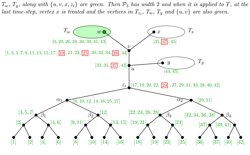
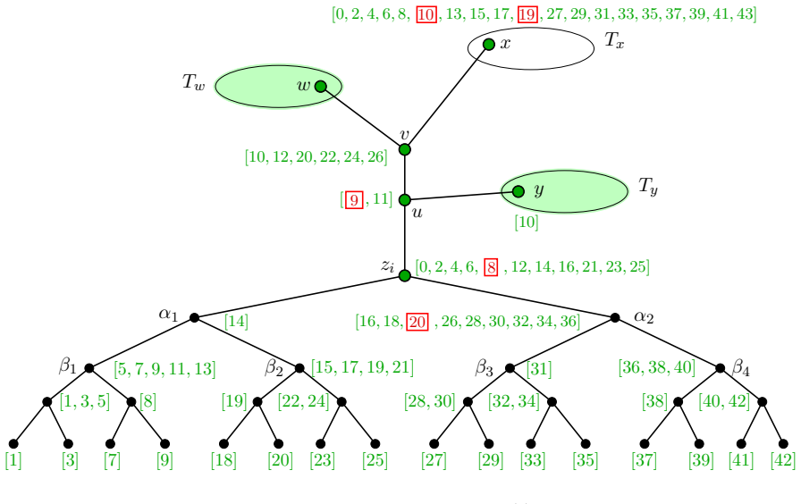
The authors prove that the discrete-time treatment number τ(BT(d)) equals 3 for 8 ≤ d ≤ 10 by characterizing the sizes of all subsets of vertices whose boundary has 3 or fewer vertices, achieving equality in the pathwidth upper bound. They give an explicit construction showing τ(BT(7)) = 2. The hereditary property implies that all larger complete binary trees have treatment number at least 3. They also construct infinite families of graphs with a cut-vertex where the treatment number depends on the number of components after removal, and use pathwidth together with vertex cuts to bound the treatment number from above while producing graphs with bounded boundary size but unbounded treatment n
What carries the argument
The complete characterization of the sizes of all vertex subsets in BT(d) whose boundary has size at most 3.
If this is right
- All complete binary trees of depth greater than 10 have treatment number at least 3.
- The pathwidth upper bound is tight for BT(d) when d equals 8, 9 or 10.
- Treatment number can depend on the number of components created by deleting a single cut vertex.
- There exist graphs with arbitrarily large treatment number whose boundary size remains bounded.
- Combining pathwidth with information about vertex cuts produces a new upper bound on treatment number.
Where Pith is reading between the lines
- The treatment number of complete binary trees may stabilize at 3 for all depths beyond 10.
- The explicit construction at depth 7 could be adapted to locate other depths where the pathwidth bound is not achieved.
- Since boundary size alone does not control treatment number, global connectivity features beyond local boundaries must matter for the parameter.
- The cut-vertex construction shows that treatment number can be made to grow by increasing the number of branches at a single vertex.
Load-bearing premise
The enumeration of all possible sizes of vertex subsets with boundary size at most 3 in BT(d) for d from 8 to 10 is complete and contains every such subset.
What would settle it
Existence of a vertex subset in BT(8) with boundary size exactly 3 whose size is missing from the enumerated list, which would show that the three-step upper bound does not hold for every possible subset.
Figures
read the original abstract
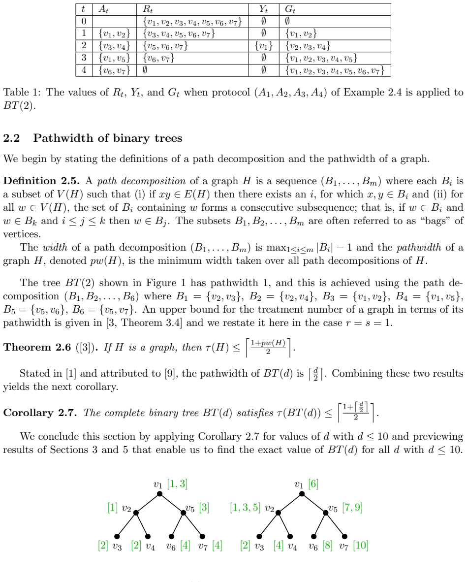
The discrete-time treatment number of a graph $H$, denoted by $\tau(H)$, was introduced in arXiv:2408.0531(3) and arises from a deterministic process in which each vertex is assigned a color at each time-step. The pathwidth upper bound $\tau(H)\leq \lceil\frac{1+pw(H)}{2}\rceil$, is shown in arXiv:2408.0531(3), where $pw(H)$ denotes the pathwidth of graph $H$. Equality holds when $H$ is the complete binary tree of depth $d$ (denoted by $BT(d)$) and $1 \le d \le 6$. In this paper, we characterize the sizes of all subsets of vertices of $BT(d)$ whose boundary has $3$ or fewer vertices and use this result to prove that $\tau(BT(d))= 3$ for $8\leq d\leq 10$; in these cases, equality also holds in the pathwidth upper bound. By the hereditary property of the treatment number, all larger complete binary trees have treatment number at least $3$. In contrast, we provide an explicit construction to show that $\tau(BT(7))=2$, while the pathwidth upper bound only shows $\tau(BT(7))\le 3.$ We construct an infinite family of graphs, each with a cut-vertex, whose treatment number depends on the number of components when the cut-vertex is removed. We use a combination of pathwidth and vertex cuts to prove another upper bound on the treatment number and use this to construct an infinite family of graphs whose boundary size is limited, but whose treatment number is unlimited.
Editorial analysis
A structured set of objections, weighed in public.
Referee Report
Summary. The paper studies the discrete-time treatment number τ(H) of graphs, focusing on complete binary trees BT(d). Building on the pathwidth upper bound τ(H) ≤ ⌈(1 + pw(H))/2⌉ from prior work, it characterizes the sizes of all vertex subsets S ⊆ V(BT(d)) with boundary |δ(S)| ≤ 3. This is used to prove τ(BT(d)) = 3 for 8 ≤ d ≤ 10 (with equality in the pathwidth bound) and, via the hereditary property, τ(BT(d)) ≥ 3 for all d ≥ 8. An explicit construction shows τ(BT(7)) = 2 (improving the pathwidth bound of 3). The paper also constructs an infinite family of graphs with a cut-vertex where τ depends on the number of components after removal, and an infinite family with bounded boundary size but unbounded τ, proved via a new upper bound combining pathwidth and vertex cuts.
Significance. If the subset characterization is complete and correct, the results determine exact values of τ(BT(d)) for d up to 10, establish new cases of tightness for the pathwidth bound, and separate τ from pathwidth and boundary size via the constructed families. The explicit construction for d=7 is a clear strength, as it is independent of the enumeration and directly exhibits a 2-treatment strategy.
major comments (1)
- [Characterization of subsets with boundary ≤3 (used in proofs for d=8–10)] The proofs that τ(BT(d))=3 for d=8,9,10 rest entirely on the claimed complete characterization of all S ⊆ V(BT(d)) with |δ(S)| ≤ 3 (used to show no 2-treatment strategy exists). The manuscript must contain an explicit, exhaustive enumeration or a rigorous proof that no admissible S is omitted; omission of even one such S would invalidate the equality claims for these depths and the hereditary extension to larger d. This is the load-bearing step for the central results on BT(d).
minor comments (2)
- [Introduction / Preliminaries] The notation for the boundary operator δ(S) and the precise definition of a k-treatment strategy should be restated in the main text (rather than only by reference to arXiv:2408.0531) to improve readability.
- [Construction for d=7] Figure captions for the explicit construction on BT(7) should include the precise sequence of color assignments at each time step to allow direct verification.
Simulated Author's Rebuttal
We thank the referee for the careful review and for highlighting the critical role of the subset characterization. We address the major comment below and will revise accordingly to strengthen the presentation.
read point-by-point responses
-
Referee: [Characterization of subsets with boundary ≤3 (used in proofs for d=8–10)] The proofs that τ(BT(d))=3 for d=8,9,10 rest entirely on the claimed complete characterization of all S ⊆ V(BT(d)) with |δ(S)| ≤ 3 (used to show no 2-treatment strategy exists). The manuscript must contain an explicit, exhaustive enumeration or a rigorous proof that no admissible S is omitted; omission of even one such S would invalidate the equality claims for these depths and the hereditary extension to larger d. This is the load-bearing step for the central results on BT(d).
Authors: We agree that the completeness of the characterization is the load-bearing step and that the manuscript must make the exhaustiveness fully rigorous. The current version derives the possible sizes of S via a structural case analysis on the positions of the (at most three) boundary vertices relative to the root and the levels of BT(d), exploiting that any admissible S must be a union of subtrees whose roots lie on a small set of paths. To address the concern directly, we will revise the relevant section to include an explicit enumeration of all admissible boundary configurations (by the depths and left/right child relations of the boundary vertices) together with a self-contained argument that these cases are exhaustive: any S with |δ(S)|≤3 must have its boundary vertices confined to at most three root-to-leaf paths, and the possible ways three (or fewer) such paths can intersect the levels of a complete binary tree are finite and fully classifiable. This revision will not change the stated results but will make the proof of completeness transparent and verifiable without external reference. revision: yes
Circularity Check
No significant circularity; new characterizations and constructions are independent of cited prior work
full rationale
The derivation relies on a new, self-contained characterization of all subsets S of BT(d) with |δ(S)| ≤ 3 (used to establish the lower bound τ(BT(d)) = 3 for d = 8–10) together with an explicit construction showing τ(BT(7)) = 2. Both are presented as original results in the paper and do not reduce to quantities defined or fitted in the cited arXiv:2408.0531(3). The pathwidth upper bound is imported from that external reference and is not re-derived here. The hereditary property is a standard graph-theoretic fact. No self-definitional steps, fitted-input predictions, or load-bearing self-citations appear.
Axiom & Free-Parameter Ledger
Reference graph
Works this paper leans on
-
[1]
H. L. Bodlaender, A partialk-arboretum of graphs with bounded treewidth,Theoretical Com- puter Science209(1998) 1-45
1998
-
[2]
Burgess, J
A.C. Burgess, J. Hawkin, A. Howse, J. Marcoux, D.A. Pike, Distance-restricted firefighting on finite graphs,Theoretical Computer Science(1061) (2026) 115658. 21
2026
-
[3]
N. E. Clarke, K. L. Collins, M. E. Messinger, A. N. Trenk, A. Vetta, Discrete-time treatment number, submitted (2025). [arXiv:2408.05313]
arXiv 2025
-
[4]
Finbow and G
S. Finbow and G. MacGillivray, The Firefighter Problem: A survey of results, directions and questions,Australasian Journal of Combinatorics43(2009) 57-77
2009
-
[5]
L. H. Harper,Global methods for combinatorial isoperimetric problems, Cambridge Stud. Adv. Math. 90, Cambridge University Press, Cambridge, 2004
2004
-
[6]
Hickingbotham, Induced subgraphs and path decompositions,The Electronic Journal of Combinatorics30(2)(2023) #P2.37
R. Hickingbotham, Induced subgraphs and path decompositions,The Electronic Journal of Combinatorics30(2)(2023) #P2.37
2023
-
[7]
Hunter and J
E. Hunter and J. Enright, The Firefighter problem with dynamic defence costs,PLOS ONE 21(2) (2026) 1-31
2026
-
[8]
Robertson and P
N. Robertson and P. D. Seymour, Graph minors I: Excluding a forest,J. Combin. Theory Ser. B35(1) (1983) 39–61
1983
-
[9]
Scheffler, Die Baumweite von Graphen als ein Maß f¨ ur die Kompliziertheit algorithmischer Probleme, Ph.D
P. Scheffler, Die Baumweite von Graphen als ein Maß f¨ ur die Kompliziertheit algorithmischer Probleme, Ph.D. thesis, Akademie der Wissenschaften der DDR, Berlin, 1989
1989
-
[10]
D. B. West,Introduction to Graph Theory, second ed., Prentice-Hall, New Jersey, 2001. 22
2001
discussion (0)
Sign in with ORCID, Apple, or X to comment. Anyone can read and Pith papers without signing in.