REVIEW 3 major objections 4 minor 38 references
Singular asymptotics for solutions of the inhomogeneous Painlev\'e II equation
T0 review · 3 major / 4 minor · reviewed 2026-08-14 · deepseek-v4-flash
Pith's one-line read For every real α and every real k with |k|>|cos(πα)|, the inhomogeneous Painlevé II equation has a real solution whose +∞ decay is an Airy correction and whose −∞ behaviour is a singular oscillation with explicit connection formulas.
desk verdict The x→+∞ extension is solid, but the local parametrix near z=1/2 contains an algebraic error that leaves the singular asymptotics and connection formulas unproven as written. read the letter →
The pith
A machine-rendered reading of the paper's core claim, the machinery that carries it, and where it could break.
The reading
What carries the argument
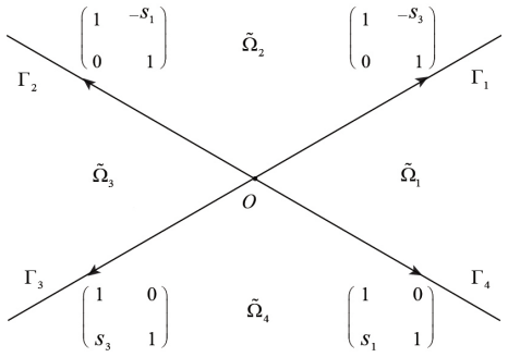
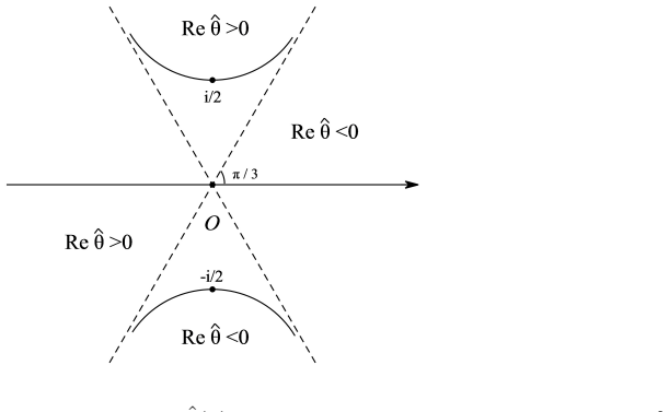
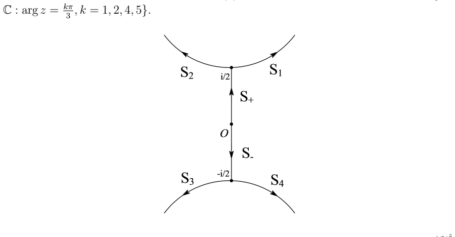
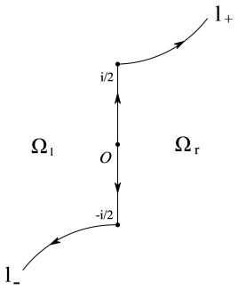
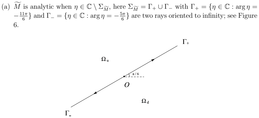
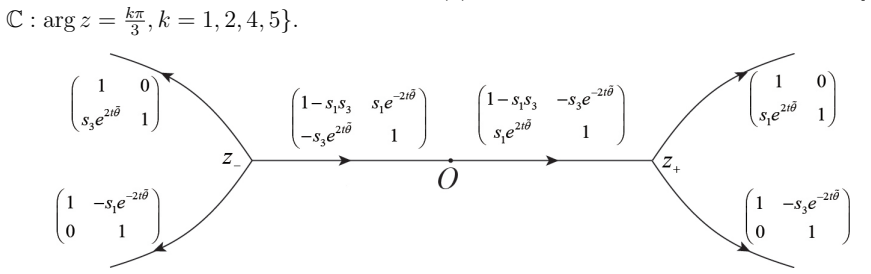
The load-bearing object is a model Riemann-Hilbert problem for a $2\times2$ matrix $M(\eta)$ with jumps on four rays and an algebraic singularity at $\eta=0$, solved explicitly by (2.6)--(2.8) in terms of the two Hankel functions $H^{(1)}_{\alpha\pm1/2}$ and $H^{(2)}_{\alpha\pm1/2}$. Because those two functions are linearly independent for every real $\alpha$, the same model works as the local parametrix at the origin when $\alpha-\tfrac12$ is an integer, a case where Bessel functions of the first kind would become linearly dependent. At the stationary point $z=\tfrac12$, the parametrix $Q^{(r)}(z)=E_r(z)P^{(r)}(z)$ is built from parabolic cylinder functions plus an explicitly singular prefactor $E_r$ with a simple pole; the resulting residue conditions (4.37)--(4.38) are fed into a dressing step $R(z)=(zI+D)\,W(z)\,\mathrm{diag}(1/(z-z_+),1/(z-z_-))$ that turns the pole problem into a solvable singular integral equation for $W$. The $(1,2)$ entry of the constant matrix $D$ gives the leading term of $u(x;\alpha)$, and the condition $1+p^2=0$ locates the poles.
What would settle it
Evaluate $\beta(z)^2/(\sqrt{t\,\zeta(z)})$ on the circle $|z-1/2|=\delta$ with $\beta(z)=(\sqrt{t\,\zeta(z)}\,(z+1/2)/(z-1/2))^{\nu}$ and $\nu=\nu_0-\tfrac12$, $\nu_0\in i\mathbb{R}$, letting $t=(-x)^{3/2}\to\infty$. If the absolute value is proportional to $t^{-1}$ rather than $O(1)$, the matching identity (4.23) fails and the residue equations (4.37)--(4.38), and hence the connection formulas (1.11)--(1.12), would need to be re-derived.
Extended reading notes
Core claim
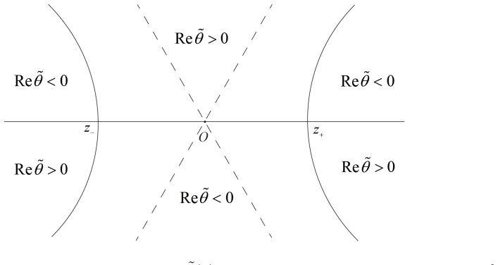
The central claim is Theorem 1: given $\alpha\in\mathbb{R}$ and $k\in\mathbb{R}$ with $|k|>|\cos(\pi\alpha)|$, there exists a real solution $u(x;\alpha)$ of $u''=2u^3+xu-\alpha$ such that $u(x;\alpha)=B(x;\alpha)+k\,\mathrm{Ai}(x)(1+O(x^{-3/4}))$ as $x\to+\infty$, where $B$ has the full expansion $B(x;\alpha)\sim(\alpha/x)\sum_{n\ge0}a_n x^{-3n}$ with $a_0=1$ and the recursion $a_{n+1}=(3n+1)(3n+2)a_n-2\alpha^2\sum_{k+l+m=n}a_k a_l a_m$; and as $x\to-\infty$, away from the zeros of the denominator, $$u(x;\$\alpha$)=\frac{\sqrt{-x}}{\sin\!\big(\tfrac23(-x)^{3/2}+\tfrac34 $d^{2}$\ln(-x)+\phi\big)}+O((-x)^{-1}),$$ with $d=\pi^{-1/2}\sqrt{\ln(k^2-\cos^2(\pi\alpha))}$ and $\phi=(3\ln2/2)d^2-\arg\Gamma(\tfrac12+\tfrac i2 d^2)-\arg(-\sin(\pi\alpha)-ki)$. The formulas are derived by constructing explicit local parametrices: a parabolic-cylinder model at the two stationary points and a model problem at the origin solved in closed form using Hankel functions, which remain linearly independent for every real $\alpha$; this is what removes the earlier restriction $\alpha-\tfrac12\notin\mathbb{Z}$. The pole locations arise from the condition $1+p^2=0$ on an explicit phase parameter $p$, producing the quantization equation (4.54).
Load-bearing premise
The derivation leans on an unverified balance: the matching of the local model near the turning point z=1/2 is assumed to stay finite as x→−∞, and if that balance fails, the formulas connecting the +∞ and −∞ behaviors would need to change.
Editorial extensions
If this is right
- The $+\infty$ asymptotic $u(x;\alpha)=B(x;\alpha)+k\,\mathrm{Ai}(x)(1+O(x^{-3/4}))$ now holds for every real $\alpha$, including the previously excluded half-integer shifts $\alpha-\tfrac12\in\mathbb{Z}$.
- For $|k|>|\cos(\pi\alpha)|$, every such solution has infinitely many poles on $(-\infty,0)$, with positions governed by the explicit quantization condition (4.54) involving the same parameters $k$ and $\alpha$.
- The connection formulas give a complete dictionary: the decay parameter $k$ at $+\infty$ determines both the logarithmic phase-shift amplitude $d$ and the phase $\phi$ at $-\infty$, so no free data is lost across the real line.
- The singular asymptotic (1.10) is uniform on intervals bounded away from poles, so the leading oscillatory envelope $\sqrt{-x}$ and the logarithmic phase $\tfrac34 d^2\ln(-x)$ are robust predictions that can be compared numerically.
- Combined with the earlier pole-free and finitely-poled cases, the classification table is now complete for all real $\alpha$ and all real $k$: pole-free solutions for $|k|\le|\cos(\pi\alpha)|$ and singular solutions with infinitely many poles otherwise.
Reading between the lines
- Editorial inference: the explicit Hankel-function model should also work at the critical value $|k|=|\cos(\pi\alpha)|$ by taking the limit $d\to0$, which would connect the finitely-poled monotonic branch at criticality to the infinitely-poled family treated here, with the phase formula degenerating in a predictable way.
- Editorial inference: the boundedness assumption behind the turning-point matching can be settled by a direct asymptotic calculation; if the ratio $\beta^2/(\sqrt{t\,\zeta})$ is in fact of order $t^{-1}$, the residue conditions would acquire extra $t$-dependence, shifting the pole quantization without necessarily destroying the leading sine formula.
- Editorial inference: the same parametrix strategy, based on Hankel functions with integer-shifted order, is likely to remove analogous exceptional-parameter restrictions in other Riemann-Hilbert problems where Bessel-function parametrices degenerate at discrete parameter values.
Signed reviews
Editorial analysis
A structured set of objections, weighed in public.
Referee Report
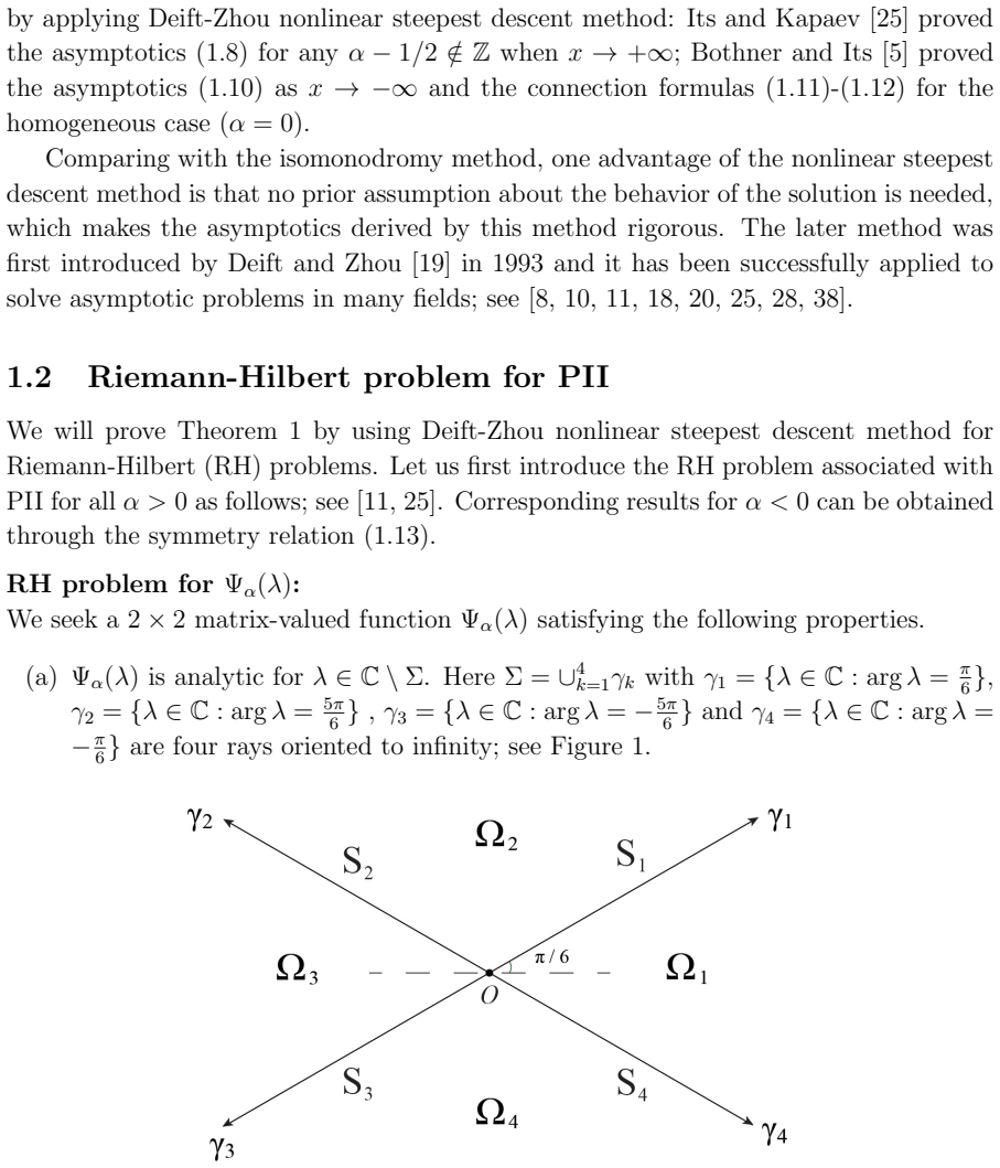
Summary. The paper studies real solutions of the inhomogeneous Painlevé II equation u''=2u^3+xu-α with α∈R\{0}, k∈R, and |k|>|cos πα|. It claims to prove, via the Deift-Zhou nonlinear steepest descent method for the associated Riemann-Hilbert problem, the asymptotics as x→+∞ (algebraic expansion plus an exponentially small Airy term), the singular asymptotics as x→-∞ (an oscillatory √(-x)/sin(...) form away from poles), and connection formulas relating the phase and logarithmic shift to k and α. The x→+∞ part extends earlier work of Its and Kapaev to all real α, while the x→-∞ part is the main new contribution and extends Bothner-Its from α=0. The proof introduces an explicit model Riemann-Hilbert problem solved in terms of Hankel functions, constructs global and local parametrices near the stationary points ±1/2 and near the origin, and uses a dressing procedure to handle the poles of the error function.
Significance. If the proof were complete, this would be a valuable contribution: it gives a purely Riemann-Hilbert derivation of the singular asymptotics and connection formulas for a family of PII solutions, matching Kapaev's isomonodromy predictions, and it closes the half-integer gap in the x→+∞ asymptotics. The model problem in Section 2 is explicit, the connection formulas are not fitted to numerical data, and the x→+∞ extension covers all real α. However, the x→-∞ analysis has a load-bearing algebraic gap in the local parametrix at z=1/2, so the main theorem as written is not established.
major comments (3)
- [Section 4.2, Eq. (4.23)] Equation (4.23) is algebraically false as stated. From (4.12) and the definitions of tilde β and tilde α in (4.22), β^2(z)/√(t ζ(z)) = t^{ν-1/2} ζ^{ν-1/2} α̃(z)^{2ν-1}. Writing ν = ν0 - 1/2 with ν0∈iR gives t^{ν0-1} ζ^{ν0-1} α̃^{2ν0-1}. On ∂U(1/2,δ), ζ is bounded away from zero, so this is O(t^{-1}), whereas the asserted right-hand side tilde β/tilde α = ζ^{2ν0} α̃^{2ν0-1} is O(1). The two sides differ by the factor t^{ν0-1} ζ^{-ν0-1}, which is not identically 1. Thus the matching condition used to pass to the lower-triangular form (4.24) is not justified.
- [Section 4.2, Eqs. (4.24)-(4.26) and (4.37)-(4.38)] The parametrix Q^(r) is built from the lower-triangular reduction in (4.24): E_r in (4.26) is chosen so that E_r P^(r) ≈ (I+O(1/t))N(z). Since (4.23) fails, the actual lower-left entry of P^(r) contains an additional t^{-ν0} ζ^{ν0} factor relative to tilde α/tilde β; consequently the residue conditions (4.37)-(4.38), the matrix D in (4.48), and the pole equation (4.54) are not established. The author should recompute the expansion of P^(r) from the Z expansion in (4.18) with the correct powers of t and ζ and adjust E_r, p, and the residue formulas accordingly.
- [Section 4.2, Eqs. (4.19) and (4.24)] The displayed transition from (4.19) to (4.24) is also not internally consistent: the (1,2) entry of the matrix in (4.24) contains a factor 1/(t ζ^2) that has no counterpart in (4.19), even after substitution of (4.23). Please derive the asymptotic expansion of P^(r) from the Z expansion in (4.18) in sufficient detail that the reader can verify the powers of t and ζ in all entries.
minor comments (4)
- [Equation (1.10)] The error terms O((-x)^{-3/2}) + O((-x)^{-1}) are redundant because the second term dominates; please state the intended uniformity statement more cleanly, for example by separating the error in the denominator approximation from the uniform remainder.
- [Introduction and Table 1] The introduction states that Hastings-McLeod solutions exist for k = sgn(α) cos(πα) for all α, but for α = n±1/2 this gives k=0 and the table marks k=cos(πα) and k=-cos(πα) as D.N.E. Please clarify which convention is intended for half-integer α.
- [Equation (4.8)] Please specify the branch of the square root in the definition of ζ(z) more explicitly; equation (4.9) fixes the local behavior, but the global branch choice in U(z_+,δ) is not stated.
- [Author affiliation] The affiliation line contains the misspelling 'Stastatics'; it should be 'Statistics'.
Circularity Check
No significant circularity: the asymptotics and connection formulas are derived from the stated Riemann–Hilbert problem with explicit Stokes data; no fitted parameter is renamed as a prediction.
full rationale
The derivation is self-contained against the Riemann–Hilbert problem in Section 1.2. The Stokes multipliers s1 = -sin(pi alpha) - k i and s3 = -sin(pi alpha) + k i are input data, and the connection formulas (1.11)-(1.12) are explicit functions of k and alpha obtained from residue conditions; no constant is fitted to the target asymptotics. The self-citations [15] and [16] are used for standard lens/parametrix technique and for prior AS/qAS results, not as justification of the new singular-asymptotics formula; the same construction is also attributed to Fokas et al. [21] and Deift-Zhou [19]. The model RH problem for M is solved explicitly in terms of Hankel functions and verified by direct asymptotics, so the parametrix is not imported as an unverified uniqueness theorem. The final formulas agree with Kapaev's earlier isomonodromy results, an independent external benchmark rather than an input. The algebraic concern about (4.23) raised in the review is a correctness issue, not circularity: even if that identity requires correction, the derivation would not become equivalent to its inputs; it would be an incomplete proof rather than a circular one.
Assumptions & free parameters
assumptions (4)
- domain assumption The Riemann-Hilbert problem for Psi_alpha is meromorphically solvable and the connection u = 2(Psi_1)_12 holds.
- domain assumption Stokes multiplier reality conditions s1 + s3 = -2 sin(pi alpha) and s1 = conj(s3).
- domain assumption Logarithmic singularities at the origin for alpha - 1/2 in N are absorbed by the algebraic behavior of the parametrix.
- standard math Standard Hankel function and parabolic cylinder identities used in Proposition 1 and Section 4.2.
Cite this review
Pith. "Pith review of Singular asymptotics for solutions of the inhomogeneous Painlev\'e II equation." pith.science (2026). https://pith.science/paper/S2BO2IJW
@misc{pith2026190805950,
  author       = {Pith},
  title        = {Pith review of: Singular asymptotics for solutions of the inhomogeneous Painlev\'e II equation},
  year         = {2026},
  howpublished = {\url{https://pith.science/paper/S2BO2IJW}},
  note         = {Machine review of arXiv:1908.05950}
}
abstract
We consider a family of solutions to the Painlev\'e II equation $$ u''(x)=2u^3(x)+xu(x)-\alpha \qquad \textrm{with } \a \in \mathbb{R} \cut \{0\}, $$ which have infinitely many poles on $(-\infty, 0)$. Using Deift-Zhou nonlinear steepest descent method for Riemann-Hilbert problems, we rigorously derive their singular asymptotics as $x \to -\infty$. In the meantime, we extend the existing asymptotic results when $x\to +\infty$ from $\a-\frac{1}{2} \notin \mathbb{Z}$ to any real $\a$. The connection formulas are also obtained.
Figures
Figures from the paper (11 more)


Reference graph
Works this paper leans on
-
[1]
M. J. Ablowitz and H. Segur, Asymptotic solutions of the Korteweg-de Vries equa- tion, Stud. Appl. Math. , 57 (1976/77), no. 1, 13–44
work page 1976
-
[2]
M. J. Ablowitz and H. Segur, Exact linearization of a Painlev´ e transcendent,Phys. Rev. Lett., 38 (1977), 1103–1106
work page 1977
-
[3]
J. Baik, P. Deift and K. Johansson, On the distribution of the length of the longest increasing subsequence of random permutations, J. Amer. Math. Soc. , 12 (1999), 1119–1178
work page 1999
-
[4]
A. Bolibruch, A. Its and A. Kapaev, On the Riemann-Hilbert-Birkhoff inverse mon- odromy problem and the Painlev´ e equations,Algebra Anal., 16 (2004), no. 1, 121– 162
work page 2004
-
[5]
T. Bothner and A. Its, The nonlinear steepest descent approach to the singular asymptotics of the second Painlev´ e transcendent,Phys. D, 241 (2012), no. 23–24, 2204–2225
work page 2012
-
[6]
Boutroux, Remarques sur les singularit´ es transcendantes des fonctions de deux variables, Bull
P. Boutroux, Remarques sur les singularit´ es transcendantes des fonctions de deux variables, Bull. Soc. Math. Fr. , 39 (1911), 296–304
work page 1911
-
[7]
Boutroux, Recherches sur les transcendantes de M
P. Boutroux, Recherches sur les transcendantes de M. Painlev e et l’´ etude asymp- totique des equations differentielles du second ordre (suite), Ann. Sci. ´Ecole Norm. Super. 31 (1914), no. 3, 99–159
work page 1914
-
[8]
R. J. Buckingham and P. D. Miller, Large-degree asymptotics of rational Painlev´ e-II functions: critical behaviour, Nonlinearity, 28 (2015), no. 6, 1539–1596
work page 2015
Show all 38 references
-
[9]
Claeys and T
T. Claeys and T. Grava, Painlev´ e II asymptotics near the leading edge of the oscil- latory zone for the Korteweg-de Vries equation in the small-dispersion limit, Comm. Pure Appl. Math. , 63 (2010), no. 2, 203–232
2010
-
[10]
Claeys and T
T. Claeys and T. Grava, Solitonic asymptotics for the Korteweg-de Vries equation in the small dispersion limit, SIAM J. Math. Anal. , 42 (2010), no. 5, 2132–2154
2010
-
[11]
Claeys, A
T. Claeys, A. B. J. Kuijlaars and M. Vanlessen, Multi-critical unitary random matrix ensembles and the general Painlev´ e II equation,Ann. of Math., 168 (2008), no. 2, 601–641
2008
-
[12]
P. A. Clarkson, Asymptotics of the second Painlev´ e equation, in Special Func- tions and Orthogonal Polynomials, 69–83, Contemp. Math., 471, Amer. Math. Soc., Providence, RI, 2008. 32
2008
-
[13]
M. G. Clerc, J. D. D´ avila, M. Kowalczyk, P. Smyrnelis and E. Vidal-Henriquez, Theory of light-matter interaction in nematic liquid crystals and the second Painlev´ e equation, Calc. Var. Partial Differential Equations , 56 (2017), no. 4, 56–93
2017
-
[14]
M. G. Clerc, E. Vidal-Henriquez, J. D. Davila and M. Kowalczyk, Symmetry break- ing of nematic umbilical defects through an amplitude equation, Phys. Rev. E , 90 (2014), 012507
2014
-
[15]
Dai and W
D. Dai and W. Y. Hu, Connection formulas for the Ablowitz-Segur solutions of the inhomogeneous Painlev´ e II equation,Nonlinearity, 30 (2017), 2982–3009
2017
-
[16]
Dai and W
D. Dai and W. Y. Hu, On the quasi-Ablowitz-Segur and quasi-Hastings-McLeod so- lutions of the inhomogeneous Painlev´ e II equation,Random Matrices Theory Appl., 7 (2018), no. 4, 1840004, 13 pp
2018
-
[17]
Deift, Orthogonal Polynomials and Random Matrices: A Riemann-Hilbert Ap- proach, Courant Lecture Notes 3, New York University, 1999
P. Deift, Orthogonal Polynomials and Random Matrices: A Riemann-Hilbert Ap- proach, Courant Lecture Notes 3, New York University, 1999
1999
-
[18]
Deift, T
P. Deift, T. Kriecherbauer, K.T-R McLaughlin, S. Venakides and X. Zhou, Uniform asymptotics for polynomials orthogonal with respect to varying exponential weights and applications to universality questions in random matrix theory, Comm. Pure Appl. Math., 52 (1999), 1335–1425
1999
-
[19]
Deift and X
P. Deift and X. Zhou, A steepest descent method for oscillatory Riemann-Hilbert problems. Asymptotics for the MKdV equation. Ann. Math. (2) , 137(1993), no. 2, 295–368
1993
-
[20]
P. A. Deift and X. Zhou, Asymptotics for the Painlev´ e II equation, Comm. Pure Appl. Math., 48 (1995), no. 3, 277–337
1995
-
[21]
A. S. Fokas, A. R. Its, A. A. Kapaev and V. Y. Novokshenov, Painlev´ e Transcen- dents: The Riemann-Hilbert Approach , Math. Surv. Monog., vol. 128, Amer. Math. Soc., Providence, RI, 2006
2006
-
[22]
Fornberg and J.A.C
B. Fornberg and J.A.C. Weideman, A computational exploration of the second Painlev´ e equation,Found. Comput. Math., 14 (2014), no. 5, 985–1016
2014
-
[23]
S. P. Hastings and J. B. McLeod, A boundary value problem associated with the second Painlev´ e transcendent and the Korteweg-de Vries equation,Arch. Rational Mech. Anal., 73 (1980), no. 1, 31–51
1980
-
[24]
E. L. Ince, Ordinary Differential Equations, New York: Dover, 1944
1944
-
[25]
A. R. Its and A. A. Kapaev, Quasi-linear Stokes phenomenon for the second Painlev´ e transcendent, Nonlinearity, 16 (2003), no. 1, 363–386. 33
2003
-
[26]
Johansson, Shape fluctuations and random matrices, Comm
K. Johansson, Shape fluctuations and random matrices, Comm. Math. Phys. , 209 (2000), 437476
2000
-
[27]
Kapaev, Global asymptotics of the second Painlev´ e transcendent,Phys
A. Kapaev, Global asymptotics of the second Painlev´ e transcendent,Phys. Lett. A, 167 (1992), no. 4, 356–362
1992
-
[28]
Kriecherbauer and K
T. Kriecherbauer and K. T. R. McLaughlin, Strong asymptotics of polynomials orthogonal with respect to Freud weights, Internat. Math. Res. Notices , 6 (1999), 299–333
1999
-
[29]
B. M. McCoy and S. Tang, Connection formulae for Painlev´ e V functions: II. The function Bose gas problem, Physica D, 20 (1986), 187–216
1986
-
[30]
J. W. Miles, On the second Painlev´ e transcendent,Proc. R. Soc. Lond. Ser. A , 361 (1978), 277–291
1978
-
[31]
P. D. Miller, On the increasing tritronqu´ ee solutions of the Painlev´ e-II equation, SIGMA, 14 (2018), 125
2018
-
[32]
F. W. J. Olver and L. C. Maximon, Bessel Functions, NIST Handbook of Mathe- matical Functions, 723–740, U.S. Dept. Commerce, Washington, DC, 2010
2010
-
[33]
R. R. Rosales, The similarity solution for the Korteweg-de Vries equation and the related Painlev´ e transcendent,Proc. R. Soc. Lond. Ser. A , 361 (1978), 265–275
1978
-
[34]
C. A. Tracy and H. Widom, Level spacing distributions and the Airy kernel, Comm. Math. Phys., 159 (1994), no. 1, 151–174
1994
-
[35]
C. A. Tracy and H. Widom, Random unitary matrices, permutations and Painlev´ e, Comm. Math. Phys. , 207 (1999), no. 3, 665-685
1999
-
[36]
W. C. Troy, The role of Painlev´ e II in predicting new liquid crystal self-assembly mechanisms, Arch. Rational Mech. Anal., 227 (2017), no. 1, 367–385
2017
-
[37]
Vanlessen, Strong asymptotics of the recurrence coefficients of orthogonal poly- nomials associated to the generalized Jacobi weight, J
M. Vanlessen, Strong asymptotics of the recurrence coefficients of orthogonal poly- nomials associated to the generalized Jacobi weight, J. Approx. Theory, 125 (2003), no. 2, 198–237
2003
-
[38]
S.-X. Xu, D. Dai and Y.-Q. Zhao, Critical edge behavior and the Bessel to Airy transition in the singularly perturbed Laguerre unitary ensemble, Comm. Math. Phys., 332 (2014), no. 3, 1257–1296. 34
2014
Reviewed August 14, 2026 · model on record in the stance chip above.
Discussion (0). Continue with ORCID to comment.