REVIEW 1 major objections 4 minor 90 references
Pattern formation with pde2path -- a tutorial
T0 review · 1 major / 4 minor · reviewed 2026-08-14 · deepseek-v4-flash
Pith's one-line read The pde2path tutorial establishes that the qswibra and cswibra routines can switch solution branches at symmetry-induced bifurcation points of multiplicity greater than one, reproducing amplitude-equation predictions in 1D, 2D, and 3D.
desk verdict A competent, candid software tutorial that deserves refereeing as a methods resource; judge it on reproducibility and usefulness, not on novelty. read the letter →
The pith
A machine-rendered reading of the paper's core claim, the machinery that carries it, and where it could break.
The reading
What carries the argument
The load-bearing object is the reduced bifurcation equation: at a bifurcation point $(u_0,\lambda_0)$ with $m$-dimensional kernel spanned by $\varphi_1,\dots,\varphi_m$ and adjoint kernel $\psi_1,\dots,\psi_m$, the tangent direction $u'(s_0)=\sum_{j=0}^m \alpha_j\varphi_j$ is found from the homogeneous quadratic system (25), or, for pitchfork-type branches, from the cubic system (27). The routines qswibra and cswibra set up these systems from second and third derivatives of $G(u,\lambda)$ projected onto the adjoint kernel, solve them by Newton loops, and store the resulting tangents; the user then selects a tangent and continues. This machinery carries the argument because it replaces the old trick of breaking the multiplicity by perturbing the domain, which hid branches such as spots, with a direct enumeration of all local branch directions. Continuous symmetries are factored out by choosing active kernel vectors (aux.ali), and phase conditions pin translations during continuation.
What would settle it
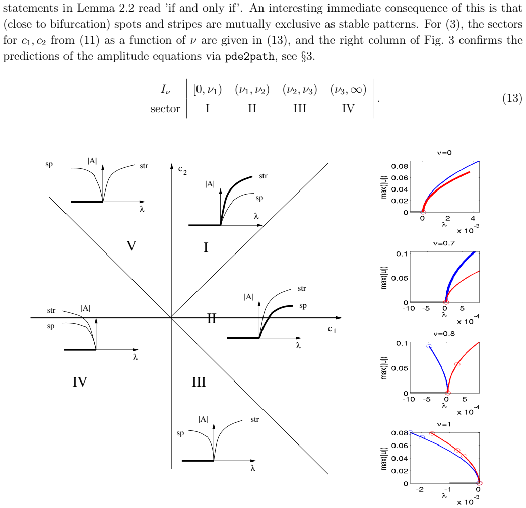
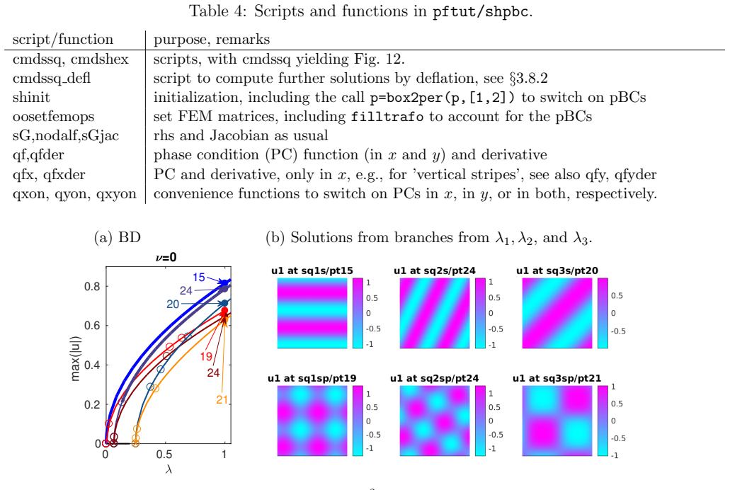
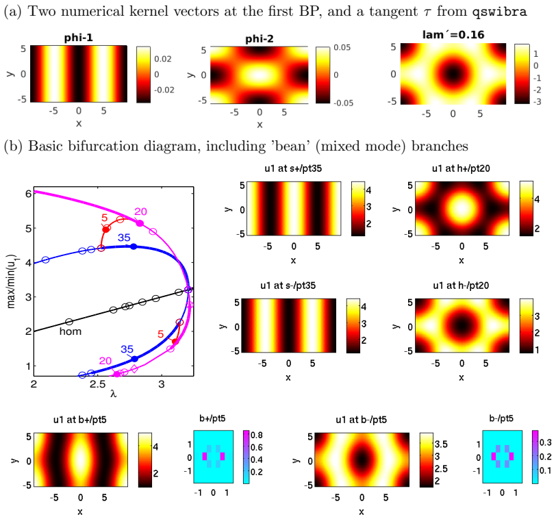
On the square-domain Swift–Hohenberg equation with $\nu=0$ and $\nu=0.7$, run cswibra at the first bifurcation point $\lambda=0$ and compare the returned tangents with the amplitude-equation solutions (12): stripes $(\alpha_1,\alpha_2)=(\pm\sqrt{\mu/c_1},0)$ and spots $(\alpha_1,\alpha_2)=(\pm\sqrt{\mu/(c_1+c_2)},\pm\sqrt{\mu/(c_1+c_2)})$. If either isotropy class is missing, or if an extra nonsymmetric tangent appears, the claim that the routine captures the true bifurcation structure fails; likewise, the claim fails if continuation of these branches swaps their predicted stability ordering from Lemma 2.2.
Extended reading notes
Core claim
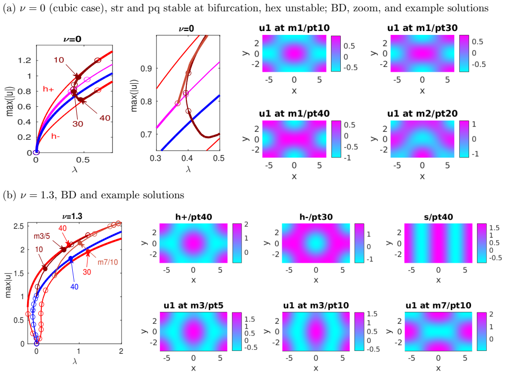
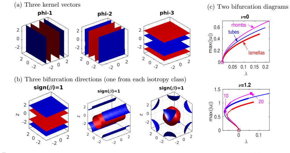
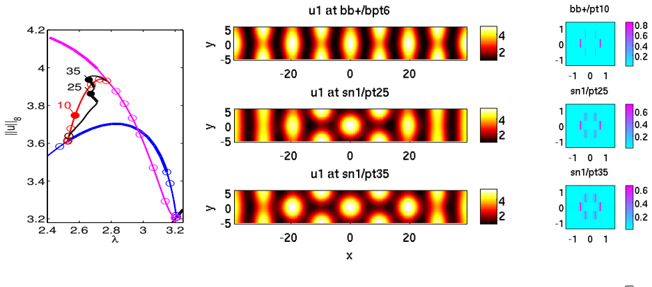
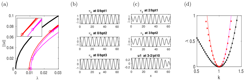
The paper's central claim is that steady bifurcation points of higher multiplicity—the typical situation in pattern-forming systems on symmetric domains—can be attacked directly instead of being perturbed away. It presents the branch-switching routines qswibra and cswibra, which solve the quadratic bifurcation equations (25) and cubic bifurcation equations (27) to obtain tangent vectors (or quadratic predictors) for every isolated bifurcating branch. Together with phase conditions for continuous symmetries, active kernel selection, and symmetry-respecting meshes, these routines reproduce, in 1D, 2D and 3D, the branch pictures predicted analytically from amplitude equations: stripes and spots on squares, hexagons and mixed modes on hexagonal domains, lamellas, tubes and rhombs on cubic lattices, and snaking branches of localized patterns. The same setup is shown to handle mass constraints, quasilinear cross-diffusion, global coupling, branch-point continuation, and pattern formation on spheres and tori.
Load-bearing premise
The finite element discretization and the numerical solution of the bifurcation equations faithfully represent the continuous PDE, so the demo branches are not artifacts of mesh asymmetry, tolerances, or software bugs.
Editorial extensions
If this is right
- Users can trust the primary bifurcation diagrams produced by pde2path on symmetric domains: on a square, the routines return both stripes and spots; on a hexagon-compatible rectangle, they return stripes, hexagons, and mixed modes, with the same stability ordering predicted by amplitude equations.
- Branch switching can be followed by continuation of secondary bifurcations, so localized patterns, snaking branches, and fronts between patterns and the trivial state can be computed in 1D, 2D, and 3D without hand-built initial guesses.
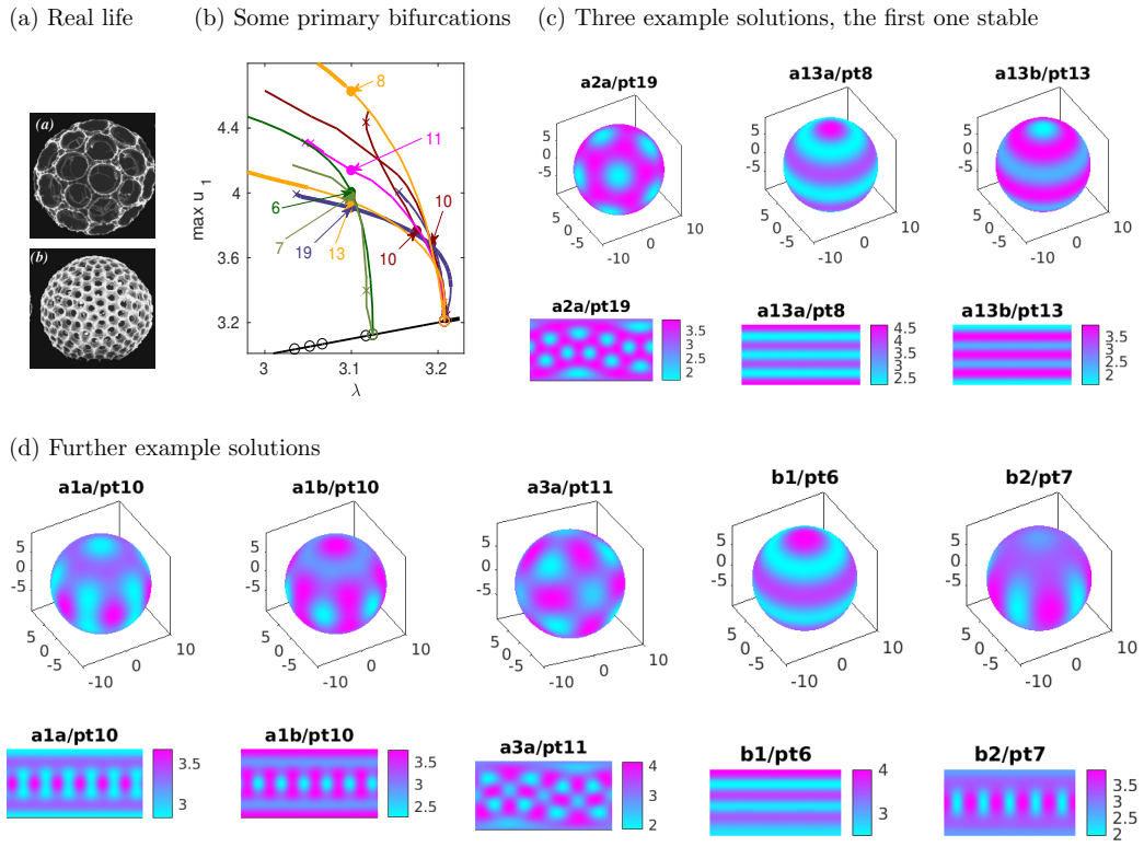
- For systems with continuous symmetries, combining active-kernel selection with phase conditions yields the same information on periodic domains, tori, and spheres, where the sphere case recovers the isotropy classes predicted by O(3)-equivariant theory.
- Auxiliary tools—branch-point continuation, deflation, and time integration for initial guesses—let the same software approximate Eckhaus curves, find disconnected branches, and reach desired patterns that are far from a known branch.
Reading between the lines
- Because the branch-switching machinery only needs the discretized equations and the derivative projections, it should transfer to other symmetry-induced multiple bifurcations—rhombic or oblique lattices, quasiperiodic domains, or systems with additional gauge symmetries—without new analysis.
- The tutorial stops where the cubic amplitude equations degenerate ($c_1=0$ or $|c_1|=|c_2|$); a natural extension is to feed fifth-order bifurcation equations into the same Newton framework and check whether the predicted vertical branches appear, which would test the determinacy threshold directly.
- On spheres, the computed branches suggest that numerical continuation can turn the curvature-dependent spot-versus-stripe observations, mostly obtained by time integration, into quantitative phase boundaries in $(R,\lambda)$ or $(R/\rho,\lambda)$ space.
Signed reviews
Editorial analysis
A structured set of objections, weighed in public.
Referee Report
Summary. This tutorial-style paper documents how the Matlab continuation package pde2path can be used for pattern-formation problems in one, two, and three space dimensions. The central technical focus is branch switching at steady bifurcation points of higher multiplicity, implemented in the routines qswibra and cswibra via quadratic and cubic bifurcation equations. The paper walks through a large set of demos: the Swift-Hohenberg equation in 1D/2D/3D, including snaking and localized patterns; the Schnakenberg system; Cahn-Hilliard and functionalized Cahn-Hilliard models with mass constraints; a chemotaxis system with quasilinear cross-diffusion; global coupling with rank-one Jacobian corrections; and pattern formation on spheres and tori. Throughout, the paper compares numerical results with analytical amplitude-equation predictions and gives practical guidance on meshes, mesh adaptation, phase conditions, deflation, and time integration as a fallback for computing isolated solutions.
Significance. If the software performs as documented, the paper is a substantial practical contribution: it makes higher-multiplicity branch switching accessible in a finite-element continuation environment and provides a large, reproducible set of demos. Its strengths are that the mathematical background is standard, the numerical demonstrations reproduce known analytical amplitude-equation results in several settings, and the software, including all demo directories, is publicly available. The paper is also honest about limitations: it explicitly states in Section 5.4 that the QBE/CBE solvers 'are not fail safe,' and Section 6.3 documents that on a sphere with a 13-dimensional kernel only a subset of branches is typically found after tuning aux.soltol and aux.isotol. This honesty is a point in favor of the paper, but it should be made visible in the abstract and introduction. The paper does not provide formal verification of the FEM discretizations or of the CBE coefficient computations; this is typical for a tutorial and does not by itself undermine the contribution.
major comments (1)
- [Abstract, §1, §5.4, §6.3] The abstract and introduction present qswibra and cswibra as the main focus of the tutorial without the substantial caveat that these routines are heuristic and can require expert tuning. Sections 5.4 and 6.3 explicitly say the methods 'are not fail safe' and that for the sphere demo 'typically only a subset of the expected branches is found' after manual adjustment of auxiliary parameters. Since the claimed added value of the tutorial is branch switching at higher-multiplicity bifurcation points, this limitation should be stated in the abstract and in Section 1, not only deep in the technical sections. I recommend adding a sentence to the effect that the routines are intended as practical tools, that exhaustive branch enumeration is not guaranteed, and that gentau and manual selection of kernel vectors remain necessary fallbacks.
minor comments (4)
- [§3.8.3, Eq. (44)] The initial guess for the BCC-to-zero front contains an evident typo: the second condition '0 z≥0' should presumably be '0 for z<0', so that the guess is nonzero on the upper half and zero on the lower half of the domain.
- [§5.3] The word 'intuitely' should be 'intuitively' in the first paragraph of Section 5.3.
- [§3.5 and §4.2] The captions and text refer to 'ten bifurcation directions' and 'four bifurcation directions' from cswibra, but only a subset is plotted; it would help the reader if the captions stated explicitly how many directions were found and how many are shown, and whether the remainder are obtained by symmetry.
- [Table 3] The description of the default isotol value and its effect on classifying solutions as isolated is somewhat terse; a one-sentence explanation of why a too-small or too-large isotol can suppress or spurioulsy create isolated solutions would make the table more usable.
Circularity Check
Self-citations are pervasive but non-load-bearing; no prediction reduces to a fit or to the cited work.
full rationale
The tutorial's analytic predictions are derived in-line from the Swift-Hohenberg equation by explicit multiple-scale amplitude-equation computations (§2), and the pde2path computations then solve the full PDE with finite elements. No fitted parameter is renamed as a prediction, and no equation used as an output is identical to an input by construction. The branch-switching routines qswibra/cswibra are presented through the QBE/CBE equations (25) and (27), with the existence of distinct branches justified by standard implicit-function arguments, and the paper explicitly warns in §5.4 and §6.3 that the routines are not fail-safe and that the sphere demo finds only a subset of branches after manual tuning. Self-citations, such as [Uec19b] for algorithmic details and [UWR14] for earlier demos, are used as pointers and background, not as the sole evidence for the numerical results. The score of 2 reflects the tutorial's heavy reliance on the author's own software and prior papers, but no actual circular reduction was found.
Assumptions & free parameters
assumptions (3)
- domain assumption Finite element discretizations converge and preserve the qualitative bifurcation structure of the continuous problems.
- standard math The quadratic and cubic bifurcation equations (QBE/CBE) characterize all relevant bifurcating branches at multiple bifurcation points.
- ad hoc to paper The pde2path software implements its documented algorithms correctly for the presented demos.
Cite this review
Pith. "Pith review of Pattern formation with pde2path -- a tutorial." pith.science (2026). https://pith.science/paper/S3GQ2PLM
@misc{pith2026190805211,
  author       = {Pith},
  title        = {Pith review of: Pattern formation with pde2path -- a tutorial},
  year         = {2026},
  howpublished = {\url{https://pith.science/paper/S3GQ2PLM}},
  note         = {Machine review of arXiv:1908.05211}
}
read the original abstract
We explain some pde2path setups for pattern formation in 1D, 2D and 3D. A focus is on new pde2path functions for branch switching at steady bifurcation points of higher multiplicity, typically due to discrete symmetries, but we also review general concepts of pattern formation and their handling in pde2path, including localized patterns and homoclinic snaking, again in 1D, 2D and 3D, based on the demo sh (Swift-Hohenberg equation). Next, the demos schnakpat (a Schnakenberg reaction-diffusion system) and chemtax (a quasilinear RD system with cross-diffusion from chemotaxis) simplify and unify previous results in a simple and concise way, CH (Cahn-Hilliard) deals with mass constraints, hexex deals with (multiple) branch points of higher degeneracy in a scalar problem on a hexagonal domain, and shgc illustrates some global coupling. The demos acS, actor, schnakS and schnaktor (the Allen-Cahn and Schnakenberg models on spheres and tori) consider pattern formation on curved surfaces, cpol considers a problem of cell polarization described by bulk-surface coupling, and bruosc (Brusselator) explains how to augment autonomous systems by a time periodic forcing. Along the way we also comment on the choice of meshes and mesh adaptation, on time integration, and we give some examples of branch point continuation and Hopf point continuation to approximate stability boundaries.
Figures


Figures from the paper (41 more)













Reference graph
Works this paper leans on
-
[1]
Alber, T
M. Alber, T. Glimm, H. G. E. Hentschel, B. Kazmierczak, and S. A. Newman. Stability of n -dimensional patterns in a generalized T uring system: implications for biological pattern formation. Nonlinearity , 18(1):125--138, 2005
2005
-
[2]
Avitabile, D.J.B
D. Avitabile, D.J.B. Lloyd, J. Burke, E. Knobloch, and B. Sandstede. To snake or not to snake in the planar Swift-Hohenberg equation. SIAM J. Appl. Dyn. Syst. , 9(3):704--733, 2010
2010
-
[3]
S. Bier, N. Gavish, H. Uecker, and A. Yochelis. Mean field approach to first and second order phase transitions in ionic liquids. PRE , 95:060201, 2017
2017
-
[4]
Burke and E
J. Burke and E. Knobloch. Localized states in the generalized S wift- H ohenberg equation. Phys. Rev. E , 73:056211, 2006
2006
-
[5]
M. Beck, J. Knobloch, D.J.B. Lloyd, B. Sandstede, and T. Wagenknecht. Snakes, ladders, and isolas of localized patterns. SIAM J. Math. Anal. , 41(3):936--972, 2009
2009
-
[6]
F. Busse. Patterns of convection in spherical shells . J. Fluid Mech. , 72:67--85, 1975
1975
-
[7]
T. K. Callahan. Turing patterns with O (3) symmetry. Phys. D , 188(1-2):65--91, 2004
2004
-
[8]
Cusseddu, L
D. Cusseddu, L. Edelstein-Keshet, J. A. Mackenzie, S. Portet, and A. Madzvamuse. A coupled bulk-surface model for cell polarisation. J. Theoret. Biol. , 481:119--135, 2019
2019
Show all 90 references
-
[9]
Cross and P.C
M.C. Cross and P.C. Hohenberg. Pattern formation outside equi\-li\-brium. Rev. Mod. Phys. , 65:854--1190, 1993
1993
-
[10]
T. K. Callahan and E. Knobloch. Symmetry-breaking bifurcations on cubic lattices. Nonlinearity , 10:1179--1216, 1997
1997
-
[11]
T. K. Callahan and E. Knobloch. Pattern formation in three-dimensional reaction-diffusion systems. Phys. D , 132(3):339--362, 1999
1999
-
[12]
T. K. Callahan and E. Knobloch. Long-wavelength instabilities of three-dimensional patterns. Phys. Rev. E , 64:036214, 2001
2001
-
[13]
Charalampidis, P.G
E.G. Charalampidis, P.G. Kevrekidis, and P.E. Farrell. Computing stationary solutions of the two-dimensional gross–pitaevskii equation with deflated continuation. Communications in Nonlinear Science and Numerical Simulation , 54:482--499, 2018
2018
-
[14]
Christlieb, N
A. Christlieb, N. Kraitzman, and K. Promislow. Competition and complexity in amphiphilic polymer morphology. Phys. D , 400:132144, 20, 2019
2019
-
[15]
Chossat, R
P. Chossat, R. Lauterbach, and I. Melbourne. Steady-state bifurcation with O (3) -symmetry. Arch. Rational Mech. Anal. , 113(4):313--376, 1990
1990
-
[16]
J. D. Crawford. Surface waves in nonsquare containers with square symmetry. PRL , 67(4):441--445, 1991
1991
-
[17]
Doelman, G
A. Doelman, G. Hayrapetyan, K. Promislow, and B. Wetton. Meander and pearling of single-curvature bilayer interfaces in the functionalized C ahn- H illiard equation. SIAM J. Math. Anal. , 46(6):3640--3677, 2014
2014
-
[18]
Dohnal, J.D.M
T. Dohnal, J.D.M. Rademacher, H. Uecker, and D. Wetzel. pde2path - V2: faster FEM and periodic domains , 2014
2014
-
[19]
Dohnal, J.D.M
T. Dohnal, J.D.M. Rademacher, H. Uecker, and D. Wetzel. pde2path 2.0 . In H. Ecker, A. Steindl, and S. Jakubek, editors, ENOC 2014 - Proceedings of 8th European Nonlinear Dynamics Conference, ISBN: 978-3-200-03433-4 , 2014
2014
-
[20]
Dohnal and H
T. Dohnal and H. Uecker. Periodic boundary conditions in pde2path , 2017
2017
-
[21]
H. de Witt. Fold and branch point continuation in pde2path -- a tutorial for systems, 2017
2017
-
[22]
H. de Witt. Beyond all order asymptotics for homoclinic snaking in a S chnakenberg system. Nonlinearity , 32:2667--2693, 2019
2019
-
[23]
W. Eckhaus. Studies in Non--Linear Stability Theory . Springer Tracts in Nat. Phil. Vol.6, 1965
1965
-
[24]
Engelnkemper, S
S. Engelnkemper, S. V. Gurevich, H. Uecker, D. Wetzel, and U. Thiele. Continuation for thin film hydrodynamics and related scalar problems. In Computational Modeling of Bifurcations and Instabilities in Fluid Mechanics , pages 459--501. Springer, 2019
2019
-
[25]
Ermentrout
B. Ermentrout. Stripes or spots? Nonlinear effects in bifurcation of reaction-diffusion equations on the square. Proc. R. Soc. Lond., Ser. A , 434(1891):413--417, 1991
1991
-
[26]
P. E. Farrell, C. H. L. Beentjes, and A. Birkisson. The computation of disconnected bifurcation diagrams, arxiv:1603.00809, 2016
2016 arXiv
-
[27]
P. E. Farrell, \' A . Birkisson, and S. W. Funke. Deflation techniques for finding distinct solutions of nonlinear partial differential equations. SIAM J. Sci. Comput. , 37(4):A2026--A2045, 2015
2015
-
[28]
W. J. Firth, L. Columbo, and A. J. Scroggie. Proposed resolution of theory-experiment discrepancy in homoclinic snaking. PRL , 99, 2007
2007
-
[29]
Gavish, K
N. Gavish, K. Hayrapetyan, G.and Promislow, and Li Yang. Curvature driven flow of bi--layer interfaces. Phys. D , 240:675--693, 2011
2011
-
[30]
a tz, and M. R\
H. Garcke, J. Kampmann, A. R\" a tz, and M. R\" o ger. A coupled surface- C ahn- H illiard bulk-diffusion system modeling lipid raft formation in cell membranes. Math. Models Methods Appl. Sci. , 26(6):1149--1189, 2016
2016
-
[31]
Golubitsky and I
M. Golubitsky and I. Stewart. The symmetry perspective . Birkh\"auser, Basel, 2002
2002
-
[32]
Glowinski and D
R. Glowinski and D. C. Sorensen. Computing the eigenvalues of the L aplace- B eltrami operator on the surface of a torus: a numerical approach. In Partial differential equations , volume 16 of Comput. Methods Appl. Sci. , pages 225--232. Springer, Dordrecht, 2008
2008
-
[33]
S. M. Houghton and E. Knobloch. Homoclinic snaking in bounded domains . Phys. Rev. E , 80:026210, 2009
2009
-
[34]
R.B. Hoyle. Pattern formation . Cambridge University Press., 2006
2006
-
[35]
Ueyama H
D. Ueyama H. Shoji, K. Yamada and T. Ohta. Turing patterns in three dimensions . Phys. Rev. E , 75:046212, 2007
2007
-
[36]
Ihrig and M
E. Ihrig and M. Golubitsky. Pattern selection with O (3) symmetry. Phys. D , 13(1-2):1--33, 1984
1984
-
[37]
Jamieson-Lane, P
A. Jamieson-Lane, P. H. Trinh, and M. J. Ward. Localized spot patterns on the sphere for reaction-diffusion systems: theory and open problems. In Mathematical and computational approaches in advancing modern science and engineering , pages 641--651. Springer, 2016
2016
-
[38]
A. L. Krause, A. M. Burton, N. T. Fadai, and R. A. Van Gorder. Emergent structures in reaction-advection-diffusion systems on a sphere. Phys. Rev. E , 97(4):042215, 13, 2018
2018
-
[39]
Kozyreff and S.J
G. Kozyreff and S.J. Chapman. Analytical results for front pinning between an hexagonal pattern and a uniform state in pattern-formation systems. PRL , 111(5):054501, 2013
2013
-
[40]
A. L. Krause, M. Ellis, , and R. A. Van Gorder. Influence of curvature, growth, and anisotropy on the evolution of T uring patterns on growing manifolds. Bull. Math. Biology , pages s11538--018--0535--y, 2018
2018
-
[41]
Kielh\"ofer
H. Kielh\"ofer. Bifurcation theory , volume 156 of Applied Mathematical Sciences . Springer, New York, second edition, 2012. An introduction with applications to partial differential equations
2012
-
[42]
H. B. Keller and W. F. Langford. Iterations, perturbations and multiplicities for nonlinear bifurcation problems. Arch. Rational Mech. Anal. , 48:83--108, 1972
1972
-
[43]
Knobloch
E. Knobloch. Spatially localized structures in dissipative systems: open problem . Nonlinearity , 21:T45--T60, 2008
2008
-
[44]
Validity of amplitude equations for nonlocal nonlinearities
Christian Kuehn and Sebastian Throm. Validity of amplitude equations for nonlocal nonlinearities. J. Math. Phys. , 59(7):071510, 17, 2018
2018
-
[45]
Chr. Kuehn. Efficient gluing of numerical continuation and a multiple solution method for elliptic PDE s. Appl. Math. Comput. , 266:656--674, 2015
2015
-
[46]
Knobloch, H
E. Knobloch, H. Uecker, and D. Wetzel. Defect--like structures and localized patterns in the cubic--quintic--septic Swift--Hohenberg equation . PRE , 100(1):012204, 2019
2019
-
[47]
Lacitignola, B
D. Lacitignola, B. Bozzini, M. Frittelli, and I. Sgura. Turing pattern formation on the sphere for a morphochemical reaction-diffusion model for electrodeposition. Commun. Nonlinear Sci. Numer. Simul. , 48:484--508, 2017
2017
-
[48]
M. Leda, V. K. Vanag, and I. R. Epstein. Instability of a three-dimensional localized spot. PRE , 80:066204, 2009
2009
-
[49]
A minimax method for finding multiple critical points and its applications to semilinear PDE s
Yongxin Li and Jianxin Zhou. A minimax method for finding multiple critical points and its applications to semilinear PDE s. SIAM J. Sci. Comput. , 23(3):840--865, 2001
2001
-
[50]
Convergence results of a local minimax method for finding multiple critical points
Yongxin Li and Jianxin Zhou. Convergence results of a local minimax method for finding multiple critical points. SIAM J. Sci. Comput. , 24(3):865--885, 2002
2002
-
[51]
P. C. Matthews. Transcritical bifurcations with O (3) symmetry. Nonlinearity , 16(4):1449--1471, 2003
2003
-
[52]
P. C. Matthews. Pattern formation on a sphere. In Dynamics and bifurcation of patterns in dissipative systems , volume 12 of World Sci. Ser. Nonlinear Sci. Ser. B Spec. Theme Issues Proc. , pages 102--123. World Sci. Publ., Hackensack, NJ, 2004
2004
-
[53]
Madzvamuse and A
A. Madzvamuse and A. Chung. The bulk-surface finite element method for reaction--diffusion systems on stationary volumes. Finnite Elements in Analysis and Design , 108:9--21, 2016
2016
-
[54]
Morgan and J.H.P
D. Morgan and J.H.P. Dawes. The S wift-- H ohenberg equation with a nonlocal nonlinearity. Physica D , 270:60--80, 2014
2014
-
[55]
A numerical approximation for the simple bifurcation problems
Zhen Mei. A numerical approximation for the simple bifurcation problems. Numer. Funct. Anal. Optim. , 10(3-4):383--400, 1989
1989
-
[56]
Numerical bifurcation analysis for reaction-diffusion equations
Zhen Mei. Numerical bifurcation analysis for reaction-diffusion equations . Springer, 2000
2000
-
[57]
A. Mielke. The G inzburg- L andau equation in its role as a modulation equation. In Handbook of dynamical systems, Vol. 2 , pages 759--834. North-Holland, 2002
2002
-
[58]
G. Moore. The numerical treatment of nontrivial bifurcation points. Numer. Funct. Anal. Optim. , 2(6):441--472 (1981), 1980
1981
-
[59]
J. D. Murray. Mathematical biology . Biomathematics. Springer-Verlag, Berlin, 1989
1989
-
[60]
Nunez-Lopez, G
M. Nunez-Lopez, G. Chacon-Acosta, and J.A. Santiago. Diffusion-driven instability on a curved surface: S pherical case revisited. Braz J Phys , (47):231--238, 2017
2017
-
[61]
Niethammer, M
B. Niethammer, M. R\"oger, and J. Velazquez. A bulk-surface reaction--diffusion system for cell polarization. Preprint, 2019
2019
-
[62]
L.M. Pismen. Patterns and interfaces in dissipative dynamics . Springer , 2006
2006
-
[63]
Press, S
W. Press, S. Teukolsky, W. Vetterling, and B. Flannery. Numerical Recipes: The Art of Scientific Computing . Cambridge University Press, 2007
2007
-
[64]
Promislow and Q
K. Promislow and Q. Wu. Existence, bifurcation, and geometric evolution of quasi-bilayers in the multicomponent functionalized cahn–hilliard equation. J. mathem. biol. , 75:443--489, 2017
2017
-
[65]
a tz and M. R\
A. R\" a tz and M. R\" o ger. Symmetry breaking in a bulk-surface reaction-diffusion model for signalling networks. Nonlinearity , 27(8):1805--1827, 2014
2014
-
[66]
Rademacher and H
J.D.M. Rademacher and H. Uecker. Symmetries, freezing, and Hopf bifurcations of modulated traveling waves in pde2path , 2017
2017
-
[67]
Rademacher and H
J.D.M. Rademacher and H. Uecker. The OOPDE setting of pde2path -- a tutorial via some Allen-Cahn models , 2019
2019
-
[68]
Swift and P.C
J. Swift and P.C. Hohenberg. Hydrodynamic fluctuations at the convective instability. Physical Review A , 15(1):319--328, 1977
1977
-
[69]
E. Siero. Nonlocal grazing in patterned ecosystems. Journal of Theoretical Biology , 436:64--71, 2018
2018
-
[70]
Stoop, R
N. Stoop, R. Lagrange, D. Terwagne, P. M. Reis, and J. Dunkel. Curvature-induced symmetry breaking determines elastic surface patterns. Nature materials , (14):337--342, 2015
2015
-
[71]
Schneider and H
G. Schneider and H. Uecker. Nonlinear PDE -- a dynamical systems approach , volume 182 of Graduate Studies Mathematics . AMS, 2017
2017
-
[72]
J. C. Tzou and L. Tzou. Spot patterns of the Schnakenberg reaction-diffusion system on a curved torus , 2019. Preprint
2019
-
[73]
A. Turing. The Turing Digital Archive, www.turingarchive.org/, AMT/C/10 , 1954
1954
-
[74]
A. Turing. Morphogen theory of phyllotaxis, Parts I - III . In P.T. Saunders, editor, Collected Works of A.M. Turing: Morphogenesis. , pages 41--118. Elsevier, Amsterdam, 1992
1992
-
[75]
H. Uecker. Optimal harvesting and spatial patterns in a semi arid vegetation system. Natural Resource Modelling , 29(2):229--258, 2016
2016
-
[76]
H. Uecker. Hopf bifurcation and time periodic orbits with pde2path -- algorithms and applications . Comm. in Comp. Phys , 25(3):812--852, 2019
2019
-
[77]
H. Uecker. Multiple bifurcation points in pde2path, 2019
2019
-
[78]
H. Uecker. Using trullekrul in pde2path -- anisotropic mesh--adaptation for some Allen--Cahn models in 2D and 3D, Preprint, arXiv 1912.11130 , 2019
1912 arXiv
-
[79]
H. Uecker. User guide on H opf bifurcation and time periodic orbits with pde2path , 2020
2020
-
[80]
H. Uecker. www.staff.uni-oldenburg.de/hannes.uecker/pde2path , 2020
2020
-
[81]
Uecker and D
H. Uecker and D. Wetzel. Numerical results for snaking of patterns over patterns in some 2D Selkov-Schnakenberg Reaction-Diffusion systems . SIADS , 13(1):94--128, 2014
2014
-
[82]
Uecker and D
H. Uecker and D. Wetzel. The pde2path linear system solvers -- a tutorial, 2017
2017
-
[83]
Uecker and D
H. Uecker and D. Wetzel. The ampsys tool of pde2path , arxiv 1906.10622, 2019
1906 arXiv
-
[84]
Uecker and D
H. Uecker and D. Wetzel. Snaking branches of planar BCC fronts in the 3D Brusselator . Phys. D , 406:132383, 2020
2020
-
[85]
Uecker, D
H. Uecker, D. Wetzel, and J.D.M. Rademacher. pde2path -- a Matlab package for continuation and bifurcation in 2D elliptic systems . NMTMA , 7:58--106, 2014
2014
-
[86]
Varea, J
C. Varea, J. L. Aragón, and R. A. Barrio. Turing patterns on a sphere. PRE , 60:4588, 1999
1999
-
[87]
D. Wetzel. Pattern analysis in a benthic bacteria-nutrient system. Math. Biosci. Eng. , 13(2):303--332, 2016
2016
-
[88]
L. Yang, M. Dolnik, A. M. Zhabotinsky, and I. R. Epstein. Pattern formation arising from interactions between T uring and wave instabilities. J. Chem. Phys. , 117(15):7259--7265, 2002
2002
-
[89]
L. Yang, A. M. Zhabotinsky, and I. R. Epstein. Stable squares and other oscillatory T uring patterns in a reaction--diffusion model. PRL , 92(19):198303--1--4, 2004
2004
-
[90]
Zelnik, H
Y. Zelnik, H. Uecker, U. Feudel, and E. Meron. Desertification by front propagation? Journal of Theoretical Biology , (418):27--35, 2017
2017
Reviewed August 14, 2026 · model on record in the stance chip above.
Discussion (0). Continue with ORCID to comment.