REVIEW 4 major objections 4 minor 34 references
Dynamic Learning Rate Decay for Stochastic Variational Inference
T0 review · 4 major / 4 minor · reviewed 2026-08-11 · deepseek-v4-flash
Pith's one-line read A signal-to-noise rule watching the variational parameter history automatically decays the SVI learning rate whenever it detects oscillation, removing the need to hand-tune the step size.
desk verdict A simple, genuinely new adaptive LR decay for SVI with promising single-run results; evidence is thin and the oscillation/curvature ambiguity is untested, but it deserves referee time. read the letter →
The pith
A machine-rendered reading of the paper's core claim, the machinery that carries it, and where it could break.
The reading
What carries the argument
The load-bearing object is the signal-to-noise ratio $\rho_i$ computed from the running sums $a_i=\sum_{j=0}^i \lambda_j$, $b_i=\sum_{j=0}^i \lambda_j^{\circ 2}$, $c_i=\sum_{j=0}^i j\lambda_j$, giving $\rho_i = \left[\frac{i(i+1)(i+2)}{12}\left(b_i-\frac{1}{i+1}a_i^{\circ 2}\right)\oslash\left(c_i-\frac{i}{2}a_i\right)^{\circ 2}-1\right]^{\circ -1}$. This is the ratio of explained to unexplained variance in the least-squares line through each variational parameter's recent history; a value below 1 means noise dominates signal. When the mean $\rho$ crosses $\rho_{\min}=1$, the rule multiplies the step by $\alpha=0.1$, resets the sums, and forbids another decay until the current interval is at least as long as the previous one. The mechanism ignores gradients entirely, so it wraps around any optimizer, including Adam, RMSprop, and AdaMax.
What would settle it
Run DLRD on an SVI problem whose ELBO landscape is strongly curved in a way that makes the optimal mean trace follow a smooth arc (for instance a banana-shaped posterior or a deep Gaussian process) while keeping the gradient noise tiny, e.g. a large batch or exact gradients. If the average $\rho$ drops below 1 and the learning rate shrinks even though the parameter is still moving steadily along the arc, with the optimization stalling as a result, the oscillation-detection mapping behind DLRD fails. Alternatively, compare the decay times against an oracle that knows the actual convergence noise level.
Extended reading notes
Core claim
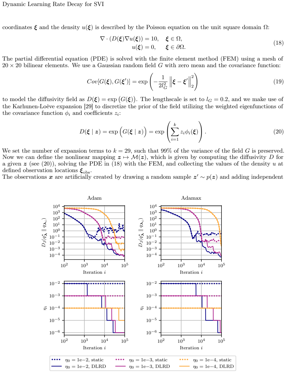
The central claim is that the oscillations a too-large learning rate causes in SVI can be recognized from the variational-parameter trajectory alone, without gradient information, and that reacting to that signal automatically is enough to achieve high accuracy across a wide range of initial learning rates. For each parameter the method fits an ordinary least-squares line through its recent iterates and forms a signal-to-noise ratio $\rho$ from the Pearson correlation of that fit; when the average $\rho$ falls below $\rho_{\min}=1$ the base learning rate is multiplied by $\alpha=0.1$ and the fit restarts. The paper demonstrates in a synthetic problem with a closed-form optimum, a Bayesian logistic-regression classifier, and a finite-element Poisson calibration that the rule prevents the oscillation plateau that stops static Adam, RMSprop, AdaMax, or SGD at high learning rates, and avoids the slow crawl of a low static rate. The authors explicitly note the method detects oscillation but not divergence, and that the reported experiments use Gaussian variational families.
Load-bearing premise
The rule assumes that a poor linear fit through the last stretch of variational parameters means the optimizer is oscillating around the optimum because the step is too large; if a curved but still productive path, a saddle region, or a noisy-but-necessary traverse also produces a low signal-to-noise ratio, the decay will fire at the wrong time and stall progress.
Editorial extensions
If this is right
- Users can start SVI with a deliberately large base learning rate to get fast initial progress and still finish at high accuracy, because the oscillation plateau is removed rather than avoided.
- The method carries over to adaptive optimizers: in the reported tests, Adam, RMSprop, and AdaMax all reach lower Jeffreys divergence with DLRD than with a static rate at the same base learning rate.
- Hand-tuned decay schedules and the SASA/SASA+ statistical tests are dominated in the tested cases: DLRD reaches the same accuracy in fewer iterations without needing a schedule exponent or stationarity window.
- The overhead is one running sum per variational parameter, comparable to Adam's, so the protection against learning-rate sensitivity does not require extra passes over data.
- Batch size does not break the mechanism: the rule improved accuracy at batch sizes 1, 8, 32, and 128 in the reported experiments.
Reading between the lines
- Beyond the paper: because the SNR criterion reads only the parameter trace, the same trigger could be attached to any iterative stochastic optimizer, including MAP estimation or VAE training, wherever the trajectory is observable; the paper only reports Gaussian variational families.
- Beyond the paper: the reset-plus-minimum-wait logic is a hysteresis that prevents back-to-back decays; this suggests a natural robustness check: test DLRD on multimodal targets where the ELBO has several basins, since a too-early decay inside one basin could lock the algorithm out of the others.
- Beyond the paper: with exact or near-exact gradients, any SNR decay would be caused by curvature rather than sampling noise, so a controlled experiment with full-batch gradients would separate the two causes, perhaps by comparing DLRD's decay times to the gradient-variance profile.
Signed reviews
Editorial analysis
A structured set of objections, weighed in public.
Referee Report
Summary. The paper proposes DLRD, a heuristic for Stochastic Variational Inference that decays the base learning rate whenever a signal-to-noise ratio computed from a linear regression of the variational-parameter history falls below a threshold. The rule is applied on top of SGD, Adam, RMSprop, and AdaMax, and is tested on a synthetic problem with an analytic optimum, Bayesian logistic regression on a public breast-cancer dataset, and a finite-element diffusivity-calibration problem. The authors report that DLRD improves accuracy relative to static learning rates and hand-picked schedules, reduces sensitivity to the initial learning rate, and also outperforms the SASA and SASA+ methods in their synthetic comparison.
Significance. If the empirical claims hold, DLRD would be a useful, low-memory complement to adaptive optimizers for SVI: it monitors only the variational-parameter trace, adds negligible per-iteration cost, and uses fixed default hyperparameters. The paper has notable strengths: the synthetic example has a closed-form optimal variational distribution, the logistic-regression example uses a public dataset, the FEM example is a realistic large-scale test, and the method is compared against SASA/SASA+ and classical Robbins-Monro schedules. However, the central evidence is currently a set of single stochastic trajectories without error bars, and the core heuristic assumption that low linear-fit SNR indicates oscillation is not directly validated. The contribution is therefore promising but not yet established at the level claimed.
major comments (4)
- [Section 3, Figures 3-8] All performance curves are single stochastic runs with no reported seeds, repeats, or error bars, yet the text repeatedly claims that accuracy is improved for all tested learning rates and optimizers (e.g., Sections 3.1-3.3). In stochastic optimization, single-run comparisons can be dominated by Monte Carlo noise, especially where curves cross or are close in final accuracy (as in Figure 7 around 3e5 iterations). Please report means and standard deviations (or quantiles) over at least 10-20 independent runs, and state the number of seeds used.
- [Section 2.3 and Appendix A] The SNR in Eq. (11) is r^2/(1-r^2) for an ordinary least-squares fit of the variational parameter against iteration, so it measures the quality of a linear fit, not oscillation specifically. A parameter moving steadily along a curved but productive path also produces large residuals around the best straight line and a low SNR, which would trigger the decay eta <- alpha*eta at the wrong time and could stall progress. This failure mode is not tested in the paper: all variational families are Gaussian, the plotted trajectories are roughly straight-then-oscillatory, and Section 4 only lists the inability to detect divergence as a limitation. Please add experiments or analyses with non-monotonic or curved parameter histories, or explicitly narrow the claims and state the conditions under which the trigger is reliable.
- [Section 2.3, Algorithm 1] The method introduces two new hyperparameters, alpha and rho_min, but no sensitivity study is reported. The claim that alpha=0.1 and rho_min=1 are default values that work without problem-dependent fine-tuning is supported only by three examples with a single setting. A small sensitivity analysis (e.g., alpha in {0.05, 0.1, 0.2} and rho_min in {0.5, 1, 2}) on at least the synthetic example would make the robustness claim concrete.
- [Section 3.1, Figure 5] The comparison with SASA and SASA+ fixes the testing interval to 1000 iterations because SVI has no epochs, but stationarity detection in SASA is sensitive to this interval choice. The conclusion that 'our DLRD approach performs better for all tested initial learning rates' is therefore not robustly established. Please vary the testing interval or justify the chosen value, and add multiple-run statistics for this comparison as well.
minor comments (4)
- [Algorithm 1 and Eq. (11)] The symbol rho is used both for the vector of per-parameter SNR values and for its mean; in Algorithm 1 the comparison 'if rho < rho_min' should explicitly use the average over parameters. Please clarify the notation consistently in the text, equations, and Algorithm 1.
- [Figure 2 caption] The caption states 'the corresponding rho_i, which is the average over the SNR vector rho_i', which is confusing because rho_i is defined in Eq. (11) as a vector. Rephrase to distinguish the vector and its scalar average.
- [Sections 3.2 and 3.3] The reference solutions are computed with Adam using a learning-rate schedule; since DLRD is compared against these references, it would be helpful to state explicitly how sensitive the reported Jeffreys divergences are to the reference-run parameters, even though the ELBO check described in Section 3.2 is a reasonable validation.
- [Section 4] The sentence 'A current limitation of our method is that it can not detect a diverging optimization progress' would read better as 'cannot detect diverging optimization progress'; also consider noting here the curvature/linearity limitation raised in the major comments.
Circularity Check
No significant circularity: the DLRD heuristic is validated against external benchmarks; its self-citations are incidental and not load-bearing.
full rationale
The paper's contribution is a heuristic learning-rate decay rule, not a derived prediction that reduces to its inputs. The trigger in Section 2.3 / Algorithm 1 is defined directly from the ordinary-least-squares SNR in Eq. (11), which Appendix A shows is just the closed-form expression r^2/(1-r^2) for the Pearson correlation of the parameter trace. The hyperparameters alpha=0.1 and rho_min=1 are fixed defaults used across all experiments; they are not fitted to the Jeffreys-divergence accuracy targets, so no measured quantity is being 'predicted' from a fitted parameter. The evaluation is external: the synthetic example has an analytically derived optimal variational distribution (Appendix B), the logistic-regression example uses a public dataset with a reference posterior computed by a long, high-batch-size run, and the FEM calibration example is an adapted benchmark problem. The two self-citations ([9] QUEENS software footnote and [28] the borrowed calibration setup) are incidental: no uniqueness theorem, ansatz, or load-bearing argument is imported from them. The paper's own stated limitations in Section 4 (inability to detect divergence, and evaluation only with Gaussian variational families) concern robustness and generality, not circular derivation. The potential weakness that low linear-fit SNR may also occur during curved but non-oscillatory progress is a correctness risk about the heuristic's trigger, not a circular step. No equation in the paper makes a target quantity equal by construction to a fitted value or to an input of the method.
Assumptions & free parameters
free parameters (2)
- alpha (learning-rate decay factor) =
0.1 (default)
- rho_min (SNR threshold) =
1 (default)
assumptions (4)
- standard math The reparameterized gradient estimator is unbiased; the score-function term has zero expectation (Eq. 7).
- ad hoc to paper Low SNR of the linear fit to the variational parameters means the optimizer is oscillating near the optimum and would benefit from a smaller step.
- domain assumption Oscillation variance around the optimum scales with the learning rate.
- standard math Robbins-Monro step-size conditions plus continuity assumptions imply stochastic gradient ascent converges to a local optimum.
Cite this review
Pith. "Pith review of Dynamic Learning Rate Decay for Stochastic Variational Inference." pith.science (2026). https://pith.science/paper/SBNBEY4T
@misc{pith2026241215745,
  author       = {Pith},
  title        = {Pith review of: Dynamic Learning Rate Decay for Stochastic Variational Inference},
  year         = {2026},
  howpublished = {\url{https://pith.science/paper/SBNBEY4T}},
  note         = {Machine review of arXiv:2412.15745}
}
read the original abstract
Like many optimization algorithms, Stochastic Variational Inference (SVI) is sensitive to the choice of the learning rate. If the learning rate is too small, the optimization process may be slow, and the algorithm might get stuck in local optima. On the other hand, if the learning rate is too large, the algorithm may oscillate or diverge, failing to converge to a solution. Adaptive learning rate methods such as Adam, AdaMax, Adagrad, or RMSprop automatically adjust the learning rate based on the history of gradients. Nevertheless, if the base learning rate is too large, the variational parameters might still oscillate around the optimal solution. With learning rate schedules, the learning rate can be reduced gradually to mitigate this problem. However, the amount at which the learning rate should be decreased in each iteration is not known a priori, which can significantly impact the performance of the optimization. In this work, we propose a method to decay the learning rate based on the history of the variational parameters. We use an empirical measure to quantify the amount of oscillations against the progress of the variational parameters to adapt the learning rate. The approach requires little memory and is computationally efficient. We demonstrate in various numerical examples that our method reduces the sensitivity of the optimization performance to the learning rate and that it can also be used in combination with other adaptive learning rate methods.
Figures


Figures from the paper (5 more)


Reference graph
Works this paper leans on
-
[1]
Stochastic Variational Inference
M. D. Hoffman, D. M. Blei, C. Wang, and J. Paisley. “Stochastic Variational Inference”. In:Journal of Machine Learning Research14.40 (2013), pp. 1303–1347. 12 Dynamic Learning Rate Decay for SVI
work page 2013
-
[2]
Variational Inference: A Review for Statisticians
D. M. Blei, A. Kucukelbir, and J. D. McAuliffe. “Variational Inference: A Review for Statisticians”. In: Journal of the American Statistical Association112.518 (Apr. 2017), pp. 859–877.doi: 10.1080/ 01621459.2017.1285773
arXiv 2017
-
[3]
An Adaptive Learning Rate for Stochastic Variational Inference
R. Ranganath, C. Wang, D. M. Blei, and E. P. Xing. “An Adaptive Learning Rate for Stochastic Variational Inference”. In:Proceedings of the 30th International Conference on Machine Learning. Ed. by S. Dasgupta and D. McAllester. Vol. 28. Proceedings of Machine Learning Research. Atlanta, Georgia, USA: PMLR, June 2013, pp. 298–306
work page 2013
-
[4]
Y. LeCun, L. Bottou, G. B. Orr, and K.-R. Müller. “Efficient BackProp”. In:Neural Networks: Tricks of the Trade. Ed. by G. B. Orr and K.-R. Müller. Berlin, Heidelberg: Springer Berlin Heidelberg, 1998, pp. 9–50. doi: 10.1007/3-540-49430-8_2
-
[5]
D. P. Kingma and J. Ba.Adam: A Method for Stochastic Optimization. 2014
work page 2014
-
[6]
Adaptive Subgradient Methods for Online Learning and Stochastic Optimization
J. Duchi, E. Hazan, and Y. Singer. “Adaptive Subgradient Methods for Online Learning and Stochastic Optimization”. In:Journal of Machine Learning Research12.61 (2011), pp. 2121–2159
work page 2011
-
[7]
T. Tieleman and G. Hinton.Lecture 6e - rmsprop: Divide the gradient by a running average of its recent magnitude. University of Toronto, 2012.url: https://www.cs.toronto.edu/~tijmen/csc321/ slides/lecture_slides_lec6.pdf
work page 2012
-
[8]
Natural Gradient Works Efficiently in Learning
S.-i. Amari. “Natural Gradient Works Efficiently in Learning”. In:Neural Computation10.2 (Feb. 1998), pp. 251–276. doi: 10.1162/089976698300017746
Show all 34 references
-
[9]
QUEENS—A general purpose framework for Uncertainty Quantification, Physics-Informed Machine Learning, Bayesian Optimization, Inverse Problems and Simulation Analytics on distributed computer systems. 2024. url: https://www.queens-py.org/
2024
-
[10]
C. M. Bishop.Pattern recognition and machine learning. Information science and statistics. New York: Springer, 2006
2006
-
[11]
A Stochastic Approximation Method
H. Robbins and S. Monro. “A Stochastic Approximation Method”. In:The Annals of Mathematical Statistics 22.3 (1951), pp. 400–407.doi: 10.1214/aoms/1177729586
1951
-
[12]
Black Box Variational Inference
R. Ranganath, S. Gerrish, and D. Blei. “Black Box Variational Inference”. In:Proceedings of the Seventeenth International Conference on Artificial Intelligence and Statistics. Ed. by S. Kaski and J. Corander. Vol. 33. Proceedings of Machine Learning Research. Reykjavik, Icelan...
2014
-
[13]
Monte Carlo Gradient Estimation in Machine Learning
S. Mohamed, M. Rosca, M. Figurnov, and A. Mnih. “Monte Carlo Gradient Estimation in Machine Learning”. In:Journal of Machine Learning Research21.132 (2020), pp. 1–62
2020
-
[14]
Rao-Blackwellisation of Sampling Schemes
G. Casella and C. P. Robert. “Rao-Blackwellisation of Sampling Schemes”. In:Biometrika 83.1 (1996), pp. 81–94
1996
-
[15]
S. M. Ross. Simulation. 4th ed. Amsterdam ; Boston: Elsevier Academic Press, 2006
2006
-
[16]
Variational Bayesian inference with stochastic search
J. Paisley, D. M. Blei, and M. I. Jordan. “Variational Bayesian inference with stochastic search”. In: Proceedings of the 29th International Coference on International Conference on Machine Learning. ICML’12. Madison, WI, USA: Omnipress, 2012, pp. 1363–1370
2012
-
[17]
D. P. Kingma and M. Welling.Auto-Encoding Variational Bayes. 2022. url: https://arxiv.org/abs/ 1312.6114
2022 arXiv
-
[18]
Variational Dropout and the Local Reparameterization Trick
D. P. Kingma, T. Salimans, and M. Welling. “Variational Dropout and the Local Reparameterization Trick”. In:Advances in Neural Information Processing Systems. Ed. by C. Cortes, N. Lawrence, D. Lee, M. Sugiyama, and R. Garnett. Vol. 28. Curran Associates, Inc., 2015
2015
-
[19]
Sticking the Landing: Simple, Lower-Variance Gradient Estimators for Variational Inference
G. Roeder, Y. Wu, and D. K. Duvenaud. “Sticking the Landing: Simple, Lower-Variance Gradient Estimators for Variational Inference”. In:Advances in Neural Information Processing Systems. Ed. by I. Guyon, U. V. Luxburg, S. Bengio, H. Wallach, R. Fergus, S. Vishwanathan, and R. G...
2017
-
[20]
M. D. Zeiler.ADADELTA: An Adaptive Learning Rate Method. 2012. url: https://arxiv.org/abs/ 1212.5701
2012 arXiv
-
[21]
Wolberg, O
W. Wolberg, O. Mangasarian, N. Street, and W. Street.Breast Cancer Wisconsin (Diagnostic). Oct
-
[22]
Parallel MCMC with Generalized Elliptical Slice Sampling
R. Nishihara, I. Murray, and R. P. Adams. “Parallel MCMC with Generalized Elliptical Slice Sampling”. In: Journal of Machine Learning Research15.61 (2014), pp. 2087–2112
2014
-
[23]
Optimization Methods for Large-Scale Machine Learning
L. Bottou, F. E. Curtis, and J. Nocedal. “Optimization Methods for Large-Scale Machine Learning”. In: SIAM Review60.2 (Jan. 2018), pp. 223–311.doi: 10.1137/16M1080173. 13 Dynamic Learning Rate Decay for SVI
2018 doi
-
[24]
Using Statistics to Automate Stochastic Optimization
H. Lang, L. Xiao, and P. Zhang. “Using Statistics to Automate Stochastic Optimization”. In:Advances in Neural Information Processing Systems. Ed. by H. Wallach, H. Larochelle, A. Beygelzimer, F. d. Alché-Buc, E. Fox, and R. Garnett. Vol. 32. Curran Associates, Inc., 2019
2019
-
[25]
Zhang, H
P. Zhang, H. Lang, Q. Liu, and L. Xiao.Statistical Adaptive Stochastic Gradient Methods. Tech. rep. MSR-TR-2020-3. Microsoft, Feb. 2020
2020
-
[26]
Efficient Gradient-Free Variational Inference using Policy Search
O. Arenz, G. Neumann, and M. Zhong. “Efficient Gradient-Free Variational Inference using Policy Search”. In:Proceedings of the 35th International Conference on Machine Learning. Ed. by J. Dy and A. Krause. Vol. 80. Proceedings of Machine Learning Research. PMLR, July 2018, pp. 234–243
2018
-
[27]
Machine learning techniques to diagnose breast cancer from image-processed nuclear features of fine needle aspirates
W. H. Wolberg, W. Street, and O. Mangasarian. “Machine learning techniques to diagnose breast cancer from image-processed nuclear features of fine needle aspirates”. In:Computer applications for early detection and staging of cancer77.2 (Mar. 1994), pp. 163–171.doi: 10.1016/03...
1994 doi
-
[28]
Dinkel, C
M. Dinkel, C. M. Geitner, G. R. Rei, J. Nitzler, and W. A. Wall.Solving Bayesian Inverse Problems With Expensive Likelihoods Using Constrained Gaussian Processes and Active Learning. 2023. url: https://arxiv.org/abs/2312.08085
2023 arXiv
-
[29]
R. G. Ghanem and P. D. Spanos.Stochastic finite elements: a spectral approach. Courier Corporation, 2003
2003
-
[30]
Variational Inference with Normalizing Flows
D. Rezende and S. Mohamed. “Variational Inference with Normalizing Flows”. In:Proceedings of the 32nd International Conference on Machine Learning. Ed. by F. Bach and D. Blei. Vol. 37. Proceedings of Machine Learning Research. Lille, France: PMLR, July 2015, pp. 1530–1538
2015
-
[31]
On the Importance of the Pearson Correlation Coefficient in Noise Reduction
J. Benesty, J. Chen, and Y. Huang. “On the Importance of the Pearson Correlation Coefficient in Noise Reduction”. In:IEEE Transactions on Audio, Speech, and Language Processing16.4 (2008), pp. 757–765. doi: 10.1109/TASL.2008.919072
2008
-
[32]
Thirteen Ways to Look at the Correlation Coefficient
J. L. Rodgers and W. A. Nicewander. “Thirteen Ways to Look at the Correlation Coefficient”. In:The American Statistician42.1 (1988), pp. 59–66
1988
-
[33]
Brookes.The Matrix Reference Manual
M. Brookes.The Matrix Reference Manual. 2020. url: http://www.ee.imperial.ac.uk/hp/staff/ dmb/matrix/intro.html. A Derivation of the Signal-to-Noise Ratio Consider the simple one-dimensional linear regression model with the iteration countj as the independent variable, a varia...
2020
-
[1995]
url: https://archive.ics.uci.edu/dataset/17
doi: 10.24432/C5DW2B. url: https://archive.ics.uci.edu/dataset/17
Reviewed August 11, 2026 · model on record in the stance chip above.
Discussion (0). Continue with ORCID to comment.