REVIEW 3 major objections 5 minor 1 cited by
Learning coupled Allen-Cahn and Cahn-Hilliard phase-field equations using Physics-informed neural operator(PINO)
T0 review · 3 major / 5 minor · reviewed 2026-08-06 · deepseek-v4-flash
Pith's one-line read This paper claims a physics-informed neural operator trained on 12 initial conditions can predict θ′ precipitate growth in Al-Cu alloys for unseen conditions with relative L2 errors of 1–6%.
desk verdict A useful feasibility demo, but the Cahn-Hilliard equation is printed wrong and no code/data exist to show the model actually solved the right PDE. read the letter →
The pith
A machine-rendered reading of the paper's core claim, the machinery that carries it, and where it could break.
The reading
What carries the argument
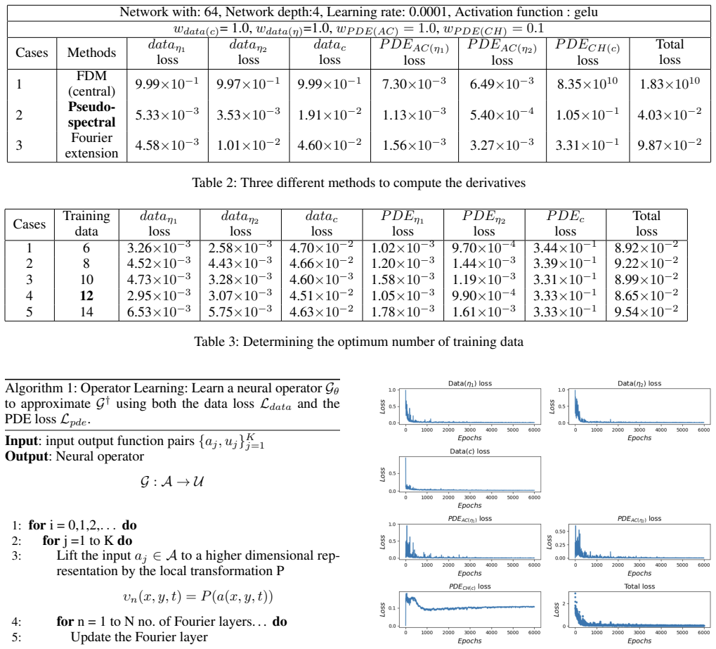
The load-bearing object is the PINO architecture: a Fourier neural operator augmented with PDE-residual loss terms. It maps the initial fields $(c,\eta_1,\eta_2)$ to the fields at later times by lifting the input, applying several Fourier layers in which an integral kernel is multiplied in frequency space, and projecting back; periodic boundary conditions are built in via fast Fourier transforms. The physics enters through a total loss combining data losses for each field with PDE residuals for the two Allen-Cahn equations and the Cahn-Hilliard equation. Derivatives are evaluated in the Fourier domain, so the fourth-order derivative of the Cahn-Hilliard term is a multiplication by $k^4$ rather than a repeated finite difference; the paper finds the choice of derivative method is decisive, with pseudo-spectral differentiation reducing the Cahn-Hilliard loss from order $10^{10}$ to order $10^{-1}$.
What would settle it
Regenerate the training data with a standard Cahn-Hilliard solver that includes the full biharmonic term $(\partial^4 c/\partial x^4 + 2\,\partial^4 c/\partial x^2\partial y^2 + \partial^4 c/\partial y^4)$, retrain the same PINO with the full operator in the PDE loss, and compare errors on the same unseen seeds; if the quoted 1–6% relative L2 accuracy does not survive, the result depends on the simplified equation.
Extended reading notes
Core claim
On its own terms, the paper establishes that a Fourier-domain PINO can solve the coupled Allen-Cahn/Cahn-Hilliard system and generalize to unseen instances. For an unseen case with supersaturated composition 0.21 and seed 1111, the relative L2 errors are $5.14\times10^{-2}$ for $c$, $1.41\times10^{-2}$ for $\eta_1$, and $1.15\times10^{-2}$ for $\eta_2$; for composition 0.23 and seed 1482 they are $5.87\times10^{-2}$, $2.21\times10^{-2}$, and $2.09\times10^{-2}$. The paper also reports that computing spatial derivatives with the pseudo-spectral method or Fourier extension instead of finite differences lowers the Cahn-Hilliard PDE loss by twelve orders of magnitude, and that the Fourier-domain derivative avoids rewriting the fourth-order equation as coupled second-order equations. On a $128\times128\times100$ domain the PINO inference time (about 0.33 s) is comparable to the numerical solver's 0.254 s, so the claimed payoff is generalization rather than per-step speed at this scale.
Load-bearing premise
The paper assumes the simplified Cahn-Hilliard equation written in Eq. 3—which omits the mixed fourth-derivative term $\partial^4 c/\partial x^2\partial y^2$—is the same physics the reference phase-field solver used to generate the training data.
Editorial extensions
If this is right
- Phase-field predictions for unseen supersaturation and seed combinations can be produced without retraining, within the range spanned by the 12 training cases.
- The fourth-order Cahn-Hilliard equation can be included directly in a physics-informed operator, without the reduction to coupled second-order equations that PINN solvers typically require.
- The differentiation scheme is a first-order decision: switching from central differences to pseudo-spectral derivatives changes the Cahn-Hilliard PDE loss by twelve orders of magnitude.
- The same PINO approach is positioned to extend to other microstructure phenomena—grain growth, coarsening, solidification, crack propagation—and to 3D simulations, where numerical solvers are far more costly.
- At the tested $128\times128$ domain size, the advantage is not speed per inference but the ability to amortize one training over many future initial conditions.
Reading between the lines
- The reported errors rest on two unseen test cases; a sweep across the full supersaturation range would show whether the 1–6% accuracy holds at the edges of the training distribution.
- The training signal may not match the conventional Cahn-Hilliard operator: Eq. 3 omits the mixed fourth derivative $\partial^4 c/\partial x^2\partial y^2$ of the biharmonic term, so a PINO trained on data from a standard solver could be fitting an inconsistent equation. This is an inference from the printed equation, not a claim the paper makes.
- Since PINO operates on Fourier modes, a natural test is zero-shot super-resolution: train at $128\times128$ and evaluate at $256\times256$; the paper lists this as future work, and the Fourier derivative machinery should make it straightforward to check.
- Speed comparisons that count only one forward pass ignore the cost of generating the 12 training trajectories; a fairer benchmark counts total time to produce a fixed number of unseen predictions, where PINO's advantage should grow.
Editorial analysis
A structured set of objections, weighed in public.
Referee Report
Summary. This manuscript trains a physics-informed neural operator (PINO) to predict the evolution of composition and order-parameter fields (c, eta_1, eta_2) for theta-prime precipitates in Al-Cu alloys, using training data generated by a phase-field solver for 25 combinations of supersaturation and seed. The model is a Fourier neural operator with a data loss plus PDE-residual losses for two coupled Allen-Cahn equations and one Cahn-Hilliard equation; derivatives are computed in the Fourier domain. Experiments report that pseudo-spectral differentiation lowers the Cahn-Hilliard PDE loss by twelve orders of magnitude relative to finite differences, and two unseen initial-condition snapshots are compared with phase-field simulations, with relative L2 errors of about 1-6%. The authors conclude that PINOs can accurately learn the physics of coupled second-order and fourth-order phase-field PDEs.
Significance. If the central issues were resolved, this would be a useful engineering demonstration: it applies PINO to a coupled, fourth-order phase-field system, shows that Fourier-domain differentiation handles the high-order operator without order reduction, and goes beyond single-instance PINN training. The comparison of differentiation methods is a practical contribution, and the two held-out cases give a sanity check. However, the paper currently provides no code or data, the evaluation is limited to two final-time snapshots, and the printed Cahn-Hilliard equation is nonstandard. The central claim therefore rests on details that the manuscript does not make verifiable.
major comments (3)
- [Methodology, Eq. (3)] As written, the Cahn-Hilliard equation is dc/dt = M(d^2/dx^2(df/dc) + d^2/dy^2(df/dc)) - 2 kappa_c M(d^4c/dx^4 + d^4c/dy^4). The standard fourth-order term for isotropic gradient energy is nabla^4 c = d^4c/dx^4 + 2 d^4c/dx^2dy^2 + d^4c/dy^4, so Eq. (3) omits the mixed derivative 2 d^4c/dx^2dy^2. Since the physics loss in Algorithm 1 is computed from Eq. (3), the model is trained to satisfy a different operator than the one used to generate the training data unless the phase-field solver also drops the mixed term. For Fourier modes with k_x approximately k_y, the printed highest-order term is half the correct value, so this is not a cosmetic typo. The authors must state unambiguously whether the actual implementation and the reference solver use the full (k_x^2 + k_y^2)^2 operator, correct Eq. (3), or specify the anisotropy that justifies the omitted term. Without code or implementation details, the reader cannot determine which residual was actually minimized.
- [Learning the evolution of theta' precipitates, Figs. 3 and 4] The generalization claim rests on two held-out initial-condition snapshots at the final time step. No error trajectory over time, no aggregate statistics over the remaining 13 unseen combinations, and no comparison with a purely data-driven FNO or with a PINN baseline are reported. In addition, Table 3 selects 12 training cases based on training loss alone; the 14-case row has a larger total loss, but no validation or test errors are shown for any data count, so the 'optimum number of training data' claim is not supported. At minimum, the authors should report the mean and spread of relative L2 errors over all held-out cases and at several time steps, and state how the training cases were split.
- [Methods to compute the derivatives, Table 2] The twelve-order-of-magnitude improvement in Cahn-Hilliard PDE loss when switching from finite differences to pseudo-spectral differentiation is reported for the training loss only (Table 2), and the comparison is between differentiation schemes implemented inside the PINO, not between solver accuracies. A large central-difference residual can arise simply because high-order finite differences are applied to near-discontinuous phase-field data, so this number does not by itself establish that the pseudo-spectral PINO solves the Cahn-Hilliard equation more accurately. The authors should report test-time PDE residuals (not just training losses) and, ideally, a convergence check under spatial resolution refinement.
minor comments (5)
- [Learning the evolution..., Table 2 caption] The hyperparameters are described inconsistently: the text says the learning rate and gamma were selected to be 0.9 and 0.001, while the Table 2 caption gives a learning rate of 0.0001. Please clarify which value was used.
- [Methodology, Eq. (6)] Equation (6) contains unclear notation, including the summation limits '1X p,i=0' and the repeated definition theta_p = eta_p^2 (p = 1, 2); the expression should be rewritten with explicit indices and a clear definition of the tensor contractions.
- [Data generation] The data format is under-specified: the training tensor is described as (N, T, X, Y) with the input being the initial condition, but it is not clear whether the operator maps the three initial fields to the full time-space solution or to the next time step. Please state the exact input-output mapping used in the neural operator.
- [References] The phase-field data generation is attributed to Kumar Makineni et al. (2017), but the cited paper appears to concern precipitation strengthening rather than phase-field modeling; please provide the actual phase-field model reference or explain how the cited work supplied the simulation data.
- [Throughout] There are several typographical and grammatical errors that should be corrected, such as 'solvinge PDEs' in the Introduction, 'spacial' in the Methods section, and formatting problems in Algorithm 1 and Table 2.
Circularity Check
No significant circularity: the PINO is trained and evaluated on held-out simulation data with a separate physics loss, and no reported error reduces by construction to a fitted input.
full rationale
The paper's derivation chain is a standard supervised-plus-physics-constrained operator-learning pipeline: generate phase-field simulation data with a solver from Kumar Makineni et al. 2017, train a PINO on 12 of 25 initial-condition/supersaturation combinations using both data loss and PDE loss, then evaluate on two unseen combinations. The reported relative L2 errors are computed from the model's output versus the held-out simulation snapshots; nothing in this procedure fits a parameter to the test data and then renames that fit a prediction. The loss weights, Fourier modes, width, depth, and learning rate are selected by trial and error, but they do not encode the reported error values. The PDE residual in Eq. 3 may omit a mixed fourth-derivative term relative to the standard Cahn-Hilliard operator, which is a correctness and reproducibility concern, not a circularity: if the printed residual does not match the data-generating equation, the physics loss would be inconsistent with the data rather than equivalent to it. The cited phase-field work is used only as a data generator, not as the justification for the claim that PINO learns the coupled PDEs. Therefore, no circular step of the types defined in the rubric is present.
Assumptions & free parameters
free parameters (3)
- loss weights wdata(c), wdata(eta), wPDE(AC), wPDE(CH) =
1, 1, 1, 0.1
- PINO architecture hyperparameters (Fourier layers, modes, width, epochs) =
4, 28, 64, about 6000
- number of training initial conditions =
12 of 25 combinations
assumptions (4)
- domain assumption The phase-field model of Kumar Makineni et al. (2017) provides high-fidelity ground truth for theta-prime growth.
- ad hoc to paper The PDE system in Eqs. 3 and 4, as written, is the correct physics of the precipitates.
- standard math Periodic boundary conditions in space are enforced by the FFT-based FNO architecture.
- domain assumption The chemical free energy and elastic energy forms in Eqs. 5 and 6 describe the theta-prime phase.
Cite this review
Pith. "Pith review of Learning coupled Allen-Cahn and Cahn-Hilliard phase-field equations using Physics-informed neural operator(PINO)." pith.science (2026). https://pith.science/paper/SE5ED3QG
@misc{pith2026250718731,
  author       = {Pith},
  title        = {Pith review of: Learning coupled Allen-Cahn and Cahn-Hilliard phase-field equations using Physics-informed neural operator(PINO)},
  year         = {2026},
  howpublished = {\url{https://pith.science/paper/SE5ED3QG}},
  note         = {Machine review of arXiv:2507.18731}
}
abstract
Phase-field equations, mostly solved numerically, are known for capturing the mesoscale microstructural evolution of a material. However, such numerical solvers are computationally expensive as it needs to generate fine mesh systems to solve the complex Partial Differential Equations(PDEs) with good accuracy. Therefore, we propose an alternative approach of predicting the microstructural evolution subjected to periodic boundary conditions using Physics informed Neural Operators (PINOs). In this study, we have demonstrated the capability of PINO to predict the growth of $\theta^{\prime}$ precipitates in Al-Cu alloys by learning the operator as well as by solving three coupled physics equations simultaneously. The coupling is of two second-order Allen-Cahn equation and one fourth-order Cahn-Hilliard equation. We also found that using Fourier derivatives(pseudo-spectral method and Fourier extension) instead of Finite Difference Method improved the Cahn-Hilliard equation loss by twelve orders of magnitude. Moreover, since differentiation is equivalent to multiplication in the Fourier domain, unlike Physics informed Neural Networks(PINNs), we can easily compute the fourth derivative of Cahn-Hilliard equation without converting it to coupled second order derivative.
Figures


Forward citations
Cited by 1 Pith paper
-
A joint voxel flow-phase field framework for ultra-long microstructure evolution prediction with physical regularization
A hybrid voxel-flow neural network plus periodic phase-field corrections predicts ultra-long microstructure evolution with lower error than pure ML and at a fraction of full-simulation cost.
Reference graph
Works this paper leans on
-
[1]
, " * write output.state after.block = add.period write newline
ENTRY address archivePrefix author booktitle chapter edition editor eid eprint howpublished institution isbn journal key month note number organization pages publisher school series title type volume year label extra.label sort.label short.list INTEGERS output.state before.all mid.sentence after.sentence after.block FUNCTION init.state.consts #0 'before.a...
-
[2]
write newline
" write newline "" before.all 'output.state := FUNCTION n.dashify 't := "" t empty not t #1 #1 substring "-" = t #1 #2 substring "--" = not "--" * t #2 global.max substring 't := t #1 #1 substring "-" = "-" * t #2 global.max substring 't := while if t #1 #1 substring * t #2 global.max substring 't := if while FUNCTION word.in bbl.in capitalize " " * FUNCT...
-
[3]
Allen, S. M.; and Cahn, J. W. 1979. A microscopic theory for antiphase boundary motion and its application to antiphase domain coarsening. Acta metallurgica, 27(6): 1085--1095
work page 1979
-
[4]
Barrett, J. W.; Blowey, J. F.; and Garcke, H. 1999. Finite element approximation of the Cahn--Hilliard equation with degenerate mobility. SIAM Journal on Numerical Analysis, 37(1): 286--318
work page 1999
-
[5]
Cahn, J. W. 1961. On spinodal decomposition. Acta metallurgica, 9(9): 795--801
work page 1961
-
[6]
Chen, N.; Lucarini, S.; Ma, R.; Chen, A.; and Cui, C. 2024. Pf-Pinns: Physics-Informed Neural Networks for Solving Coupled Allen-Cahn and Cahn-Hilliard Phase Field Equations. Available at SSRN 4761824
work page 2024
-
[7]
Kumar Makineni, S.; Sugathan, S.; Meher, S.; Banerjee, R.; Bhattacharya, S.; Kumar, S.; and Chattopadhyay, K. 2017. Enhancing elevated temperature strength of copper containing aluminium alloys by forming L12 Al3Zr precipitates and nucleating ^ precipitates on them. Scientific reports, 7(1): 1--9
work page 2017
-
[8]
Li, Z.; Kovachki, N.; Azizzadenesheli, K.; Liu, B.; Bhattacharya, K.; Stuart, A.; and Anandkumar, A. 2020. Fourier neural operator for parametric partial differential equations. arXiv preprint arXiv:2010.08895
arXiv 2020
Show all 19 references
-
[9]
Li, Z.; Zheng, H.; Kovachki, N.; Jin, D.; Chen, H.; Liu, B.; Azizzadenesheli, K.; and Anandkumar, A. 2021. Physics-informed neural operator for learning partial differential equations. ACM/JMS Journal of Data Science
2021
-
[10]
Liu, C.; and Shen, J. 2003. A phase field model for the mixture of two incompressible fluids and its approximation by a Fourier-spectral method. Physica D: Nonlinear Phenomena, 179(3-4): 211--228
2003
-
[11]
Lu, L.; Jin, P.; Pang, G.; Zhang, Z.; and Karniadakis, G. E. 2021. Learning nonlinear operators via DeepONet based on the universal approximation theorem of operators. Nature machine intelligence, 3(3): 218--229
2021
-
[12]
Mattey, R.; and Ghosh, S. 2022. A novel sequential method to train physics informed neural networks for Allen Cahn and Cahn Hilliard equations. Computer Methods in Applied Mechanics and Engineering, 390: 114474
2022
-
[13]
Paszke, A.; Gross, S.; Massa, F.; Lerer, A.; Bradbury, J.; Chanan, G.; Killeen, T.; Lin, Z.; Gimelshein, N.; Antiga, L.; et al. 2019. Pytorch: An imperative style, high-performance deep learning library. Advances in neural information processing systems, 32
2019
-
[14]
Raissi, M.; Perdikaris, P.; and Karniadakis, G. E. 2019. Physics-informed neural networks: A deep learning framework for solving forward and inverse problems involving nonlinear partial differential equations. Journal of Computational physics, 378: 686--707
2019
-
[15]
Rezaei, S.; Harandi, A.; Moeineddin, A.; Xu, B.-X.; and Reese, S. 2022. A mixed formulation for physics-informed neural networks as a potential solver for engineering problems in heterogeneous domains: Comparison with finite element method. Computer Methods in Applied Mechanic...
2022
-
[16]
G.; Al Majed, H.; and Huerta, E
Rosofsky, S. G.; Al Majed, H.; and Huerta, E. 2023. Applications of physics informed neural operators. Machine Learning: Science and Technology, 4(2): 025022
2023
-
[17]
Sun, Z. Z. 1995. A second-order accurate linearized difference scheme for the two-dimensional Cahn-Hilliard equation. Mathematics of Computation, 64(212): 1463--1471
1995
-
[18]
Wang, S.; Wang, H.; and Perdikaris, P. 2021. Learning the solution operator of parametric partial differential equations with physics-informed DeepONets. Science advances, 7(40): eabi8605
2021
-
[19]
L.; and Zhao, J
Wight, C. L.; and Zhao, J. 2020. Solving Allen-Cahn and Cahn-Hilliard equations using the adaptive physics informed neural networks. arXiv preprint arXiv:2007.04542
2020 arXiv
Reviewed August 6, 2026 · model on record in the stance chip above.
Discussion (0). Sign in to comment.