REVIEW 3 major objections 7 minor 36 references
Use of Bayesian Inference to Diagnose Issues in Experimental Measurements of Mechanical Disk Resonators
T0 review · 3 major / 7 minor · reviewed 2026-08-07 · deepseek-v4-flash
Pith's one-line read Bayesian modeling of the split-photodiode nonlinearity recovers disk-resonator decay constants up to 25% more accurately than simple exponential fitting, and fits ringdowns the old method discarded.
desk verdict Genuinely useful Bayesian framework for ringdown analysis with a real novelty in the photodiode model, but the abstract's 25% claim is unsupported and the likelihood has a documented noise-floor limitation. read the letter →
The pith
A machine-rendered reading of the paper's core claim, the machinery that carries it, and where it could break.
The reading
What carries the argument
The load-bearing object is the analytic signal model M3 together with the two-component noise likelihood. M3 starts from a Gaussian-beam model of a split photodiode with a finite gap, where the differential voltage is a difference of error functions; expanding that response as a Taylor series in the beam position $\mu$ to order $T$ gives $V_{S,T} = \sum_{k=0}^{T} C_k \mu^k$, with coefficients fixed by the gap and beam size. Demodulating at the mode-pair midpoint frequency and low-pass filtering casts the squared readout as a sum of beat harmonics, $s_3^2(t) = X_0 + X_1 \cos(\Delta\omega t + \Delta\varphi) + \cdots + X_T \cos(T\Delta\omega t + T\Delta\varphi)$, whose coefficients carry powers of the decaying amplitudes $A_1, A_2$ and the decay constants $\tau_1, \tau_2$. The likelihood treats each ringdown sample as Gaussian with variance $\xi_i^2 = s(t_i)^2 \xi_A^2 + \xi_S^2$, adding an amplitude-proportional relative-intensity-noise term to a stationary electronic-noise term, and nested sampling with normalizing flows is used to compute posteriors and Bayes factors for model comparison.
What would settle it
Generate 50 simulated ringdowns with the full numerical photodiode model (M2) and add a hard FFT noise floor so that the signal drops below it in the second half of each record; then run the M3, $T=7$ inference. If the posterior medians for $\tau_1$ and $\tau_2$ are systematically displaced from the injected values, or if the 3-$\sigma$ intervals exclude the truth in more than a few percent of cases, the two-component Gaussian likelihood fails for low-amplitude tails and the claimed accuracy gain does not generalise.
Extended reading notes
Core claim
The central discovery, on the paper's own terms, is that the bias in ringdown parameter estimation comes from two effects the old analysis ignored: the Gaussian laser spot sweeping across the photodiode gap produces an amplitude-dependent, harmonic-generating response, and the readout noise is not stationary but scales with the instantaneous signal. The paper shows that modeling both effects with M3 and a two-component Gaussian likelihood recovers the true injected $\tau_1$ and $\tau_2$ in simulations where the simple model M1 is often biased—more than half of M1's posteriors exclude the true value, while M3 excludes it in only four ringdowns, all of which dip below the relative-intensity-noise floor. On real data the same framework yields tighter, more consistent mechanical-loss estimates across mode families and eliminates the spurious outliers and outright failures of the original method, including fits to six ringdowns that had previously been unanalysable.
Load-bearing premise
The load-bearing premise is that every ringdown data point is an independent Gaussian random variable whose variance is the signal squared times an amplitude-noise term plus a stationary-noise term; in reality each point is the peak of a 0.2-second FFT power spectrum, so the statistics are extreme-value rather than Gaussian and the model breaks down once the signal falls to the noise floor.
Editorial extensions
If this is right
- Previously discarded single-decay ringdowns—six in this dataset—can be fitted without special handling, yielding posterior distributions for both $\tau_1$ and $\tau_2$ instead of failing.
- Mechanical-loss estimates become more tightly clustered across repeated measurements of the same mode family, and the spurious outliers in $1/Q_2$ seen with the original method disappear.
- The Bayes factor between M1 and M3 tells the experimenter when a given measurement needs the nonlinear readout model and when the simple exponential model suffices, so model complexity can be matched to oscillation amplitude.
- Up to 25% better accuracy in $\tau_1$ and $\tau_2$ translates directly into smaller uncertainties in the inferred coating loss $\phi(f) = 1/(\pi f \tau)$, and hence in predicted coating Brownian thermal noise.
- Residuals and posterior widths from the Bayesian fit expose amplitude-dependent distortions in the apparatus that the old analysis hid, turning the fitter into a diagnostic tool.
Reading between the lines
- Because each ringdown data point is the maximum of a 0.2 s FFT power spectrum, replacing the Gaussian likelihood with an extreme-value model for that maximum is a direct way to remove the noise-floor bias the paper itself documents in Appendix B.1; this is my inference, not a claim the paper makes.
- The same Taylor-expansion-of-the-error-function trick should transfer to any optical-lever or split-detector measurement where a Gaussian spot scans across a gap, so the framework is likely applicable beyond disk resonators to other mechanical loss measurements.
- Switching the readout from FFT-bin maxima to heterodyne or lock-in demodulation, which the authors mention, would simplify the likelihood and reduce the computational cost of the nested-sampling analysis while sidestepping the noise-floor problem.
- The model-comparison logic could be used diagnostically in reverse: a low-amplitude ringdown that strongly prefers M3 may signal a misaligned beam, an unexpected beam size, or an asymmetric photodiode response, giving a data-driven check on apparatus alignment.
Editorial analysis
A structured set of objections, weighed in public.
Referee Report
Summary. The manuscript presents a Bayesian framework for extracting the two decay constants tau1 and tau2 from GeNS ringdown measurements of coated disk resonators used in gravitational-wave coating loss studies. Three signal models are considered: a traditional two-exponential model (M1), a numerical split-photodiode model (M2) that includes the Gaussian beam profile and photodiode gap nonlinearity, and an analytic power-series approximation (M3) that enables fast likelihood evaluation. The likelihood in Eq. (24) combines stationary and amplitude-proportional (RIN-like) Gaussian noise. The models are validated on 50 simulated ringdowns generated with M2 and applied to 47 real ringdowns, with model comparison performed via nested sampling (nessai) and Bayes factors. The paper claims up to 25% improvement in estimation accuracy over traditional methods, especially for larger oscillation amplitudes, and reports that six previously unfittable ringdowns can now be analyzed without adjustment.
Significance. The framework addresses a genuine and consequential problem: photodiode nonlinearity and RIN noise create model misspecification that biases conventional exponential fits, and the paper offers a physically motivated correction with principled model comparison. The analytic M3 construction, the two-component noise model with standardized residual diagnostics, and the public implementation (bayesbeat) with a data release are notable strengths, as is the unusually candid documentation of failure modes (four biased simulations, one tau1/tau2 swap, and prior-width sensitivity in Appendix B.1). If the accuracy claims hold after the requested quantification, this is a useful contribution to the mechanical-loss and coating thermal noise community and to the instrumentation readership of Classical and Quantum Gravity.
major comments (3)
- [Abstract; Section 3.2 (Figure 4); Section 5.2 (Figure 10)] The abstract's headline claim of 'improvements in estimation accuracy by up to 25%' is not supported by the accuracy metrics reported in the paper. The only 25% figure in the manuscript is in Section 3.2 (Figure 4), where it quantifies the difference between the predicted amplitudes of the T=1 and T=7 signal models, not the error in the inferred decay constants. The accuracy comparison in Figure 10 is reported qualitatively ('M3 is consistently closer to the true value'), with no percentage improvement, and the text also states that at lower amplitudes neither model is favoured. Please report a quantitative accuracy metric (e.g., median or 90th percentile of |tau_hat - tau_true|/tau_true across the 50 injections, binned by amplitude) or reword the abstract so that the 25% figure is attributed to model-output differences rather than to estimation accuracy.
- [Eq. (24); Eq. (2); Appendix B.1; Section 7] The likelihood in Eq. (24) treats each ringdown sample as an independent Gaussian with variance s(t_i)^2 xi_A^2 + xi_S^2, but each d(t_i) in Eq. (2) is the maximum of an FFT power spectrum over a 0.2 s window; its distribution is an extreme-value statistic with a positive noise floor that does not vanish as s -> 0. The authors themselves document the consequence: Appendix B.1 reports biased tau estimates in four of the 50 simulated ringdowns when the signal falls below the FFT/RIN noise floor, including one case with a tau1/tau2 swap, and Section 7 concedes that the model does not account for the FFT noise floor. This is precisely the regime relevant to the claim in Section 6 that six previously discarded real ringdowns, described in Appendix B.3 as low-amplitude and often single-decay signals, 'can now be reliably analysed.' As it stands, the unconditional 'superior estimation accuracy' of the abstract is not established for these low-SNR tails. I request either a quantitative assessment of the bias for the affected real ringdowns (e.g., a posterior predictive check that includes a noise-floor term, or an analysis demonstrating that those ringdowns do not enter the low-SNR regime) or a scope-limited wording of the claim.
- [Section 5.2; Eq. (13); Section 3.2] The simulated-data validation is largely a self-consistency check within one model family: the injections are generated with M2 (Eq. (13)) and analyzed with M3 (Section 3.2), an analytic approximation of the same photodiode model. The recovery of the injected tau values therefore demonstrates internal consistency of the signal-model family rather than the adequacy of the signal model against an independent ground truth; the comparison that matters for the paper's improvement claim is M3 versus M1, and both share the same, possibly misspecified, Gaussian likelihood of Eq. (24). A concrete strengthening would be to inject simulated data using the extreme-value statistic of Eq. (2) including the noise floor, or to validate M3 against a measured photodiode response such as the scan in Figure 2b, which would test the absolute accuracy of the inferred decay constants rather than only the relative improvement over M1.
minor comments (7)
- [Section 4.2, after Eq. (21)] The two noise components are mislabeled in the text: 'The first, nA is stationary Gaussian noise' and 'The second, nA is amplitude dependent noise' both refer to nA, whereas in Eq. (22) the multiplicative amplitude-dependent component is nA and the stationary component is nS; the text should be corrected to match Eq. (22).
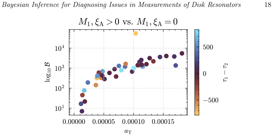
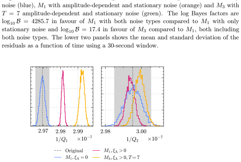
- [Section 5.1 and Figure 5 caption] The condition 'xi_A < 0' appears twice ('allowing xi_A < 0 has minimal effects of the signal fit' and 'with only stationary noise versus (xi_A = 0) stationary and amplitude dependent noise (xi_A < 0)'); the intended condition is xi_A > 0, and the sign flip will confuse readers.
- [Eq. (17)] As typeset, the first and third terms on the right-hand side of Eq. (17) are identical and opposite in sign, so the 3*omega_1 contribution cancels exactly; presumably one sign is a typographical error. Since the full expressions for M3 are only given in the bayesbeat code, this displayed equation should be corrected so that the derivation is checkable from the paper alone.
- [Section 5.2, near Figure 8] The phrase 'at lower amplitudes neither model is favoured (log10 B = 1)' is inconsistent with the Jeffreys scale defined in Section 4, where log10 B > 1 is strong evidence in favor of one model; the scatter in Figure 8 suggests values near zero at low amplitude, so this should presumably read 'log10 B is close to 0'.
- [Section 1 and Reference [1]] The in-text claim that 'the landmark detection of GW150914_095045 in 2015 [1]' is supported by reference [1], which is the 2016 Living Reviews article by Abbott (arXiv:1304.0670), not the GW150914 discovery paper; the correct citation is Abbott et al., Phys. Rev. Lett. 116, 061102 (2016). In addition, the sentence ending '...calculated (see Figure 1). to the isotropy of the substrate...' appears to be missing the word 'Due' at the start of the second clause.
- [Appendix A.1] The beat-frequency prior is set using the same data that are subsequently analyzed ('This is achieved by applying a fourth-order low-pass butter filter, computing the FFT of the data, and then finding any frequencies...'), which is a double use of the data in the evidence calculation; given the enormous Bayes factors the conclusions are unlikely to change, but this data-driven prior should be acknowledged or fixed independently of the data.
- [Appendix C and Figure 10 caption] Two small presentation issues: in Figure 10 the caption has an unclosed parenthesis ('M3 with T = 7 (orange when analysing 50 simulated ringdowns'), and in Appendix C the text reads 'the analyses with M3 taken longer' instead of 'take longer'.
Circularity Check
No construction-level circularity: the tau estimates come from a likelihood fit, and the real-data/Vajente comparison supplies an external baseline; the M2-generated simulations make the Section 5 validation partly a self-consistency check, and the FFT noise-floor limitation (Section 7, Appendix B.1) narrows but does not circularize the accuracy claim.
full rationale
The paper's central claim is that Bayesian inference with M3 (T=7) plus a two-component noise model recovers tau1 and tau2 more accurately than simplified M1. This is not circular at the construction level: the tau values are free parameters in the likelihood (Eq. 24) and are inferred from data; no fitted parameter is relabelled as a prediction, and no equation defines the target result in terms of itself. The main soft spot is that the simulated truth is generated from M2 (Eq. 13), while M3 is derived from M2 by Taylor expansion (Eqs. 15-16), so Section 5's recovery of injected taus is partly a self-consistency test within the M2/M3 model family rather than an independent validation. The authors concede this limitation: Appendix B.1 reports four simulated ringdowns with biased tau estimates (including one tau1/tau2 swap) when the signal falls below the FFT noise floor, and Section 7 states that the model 'does not account for the noise floor that results from applying the FFT' and that 'the data will no longer be Gaussian' in that regime. This limits the scope of the claimed superior accuracy in low-amplitude tails, but it is a statistical-model misspecification, not circularity. The paper also provides external anchors: M1 is the published Vajente model, real ringdowns are compared with Vajente's original estimates, and six previously 'unfittable' ringdowns are analysed without adjustment. Self-citations (nessai, bayesbeat, and Tait et al. [9]) are to software and stated modelling choices that are code-reproduced or derived in the text; no load-bearing uniqueness theorem is imported. The abstract's 'up to 25%' improvement figure traces to Figure 4, which compares model amplitudes for T=3,5,7 versus T=1 rather than directly reporting tau-recovery statistics; this is a presentation weakness, not a circular derivation. Verdict: no circular step identified; score 2 reflects minor self-citations and the self-consistency validation caveat.
Assumptions & free parameters
free parameters (5)
- Truncation order T =
7
- Beat-frequency prior width δ =
0.05 Hz for real data, 0.2 rad for simulated data
- Photodiode gap xg =
0.25 mm
- Beam radius σ =
1.5 mm
- Noise parameters ξA and ξS =
Inferred per ringdown
assumptions (6)
- domain assumption The ringdown signal is a superposition of exactly two exponentially decaying sinusoids from a degenerate mode pair (Eq. 3).
- domain assumption The photodiode voltage is the difference of Gaussian-beam powers integrated over two half-planes with a finite gap (Eqs. 7-12).
- domain assumption The FFT bin value equals the power of the signal components inside that bin, and taking the maximum over the spectrum selects the mode-pair beat (Eq. 13).
- domain assumption M3's low-pass filtering discards all terms above T(ω1-ω2), and the Taylor series truncated at order T is accurate (Eqs. 18-19).
- domain assumption Noise is stationary plus amplitude-proportional Gaussian noise, uncorrelated between samples (Eqs. 22-24).
- standard math Standard Taylor expansion and integration of the error function.
Cite this review
Pith. "Pith review of Use of Bayesian Inference to Diagnose Issues in Experimental Measurements of Mechanical Disk Resonators." pith.science (2026). https://pith.science/paper/SLGX43W3
@misc{pith2026250517346,
  author       = {Pith},
  title        = {Pith review of: Use of Bayesian Inference to Diagnose Issues in Experimental Measurements of Mechanical Disk Resonators},
  year         = {2026},
  howpublished = {\url{https://pith.science/paper/SLGX43W3}},
  note         = {Machine review of arXiv:2505.17346}
}
abstract
Gravitational wave detectors, such as LIGO, are predominantly limited by coating Brownian thermal noise (CTN), arising from mechanical losses in the Bragg mirror coatings used on test-mass optics. Accurately characterizing and minimizing these losses is crucial for enhancing detector sensitivity. This paper introduces a general mathematical and statistical framework leveraging Bayesian inference to precisely analyse mechanical ring-down measurements of disk resonators, a standard method for quantifying mechanical loss in coating materials. Our approach presents a refined model that fully captures the non-linear behaviour of beam spot motion on split photodiode sensors, significantly improving upon traditional simplified exponential-decay methods. We achieve superior estimation accuracy for decay constants ($\tau_1$ and $\tau_2$), especially for measurements exhibiting larger oscillation amplitudes. Specifically, we observe improvements in estimation accuracy by up to 25$\%$ over traditional methods, with strong Bayesian evidence favouring our framework. Our simulations and experimental validations reveal that previously discarded measurements due to fitting inaccuracies can now be reliably analysed, maximizing the use of available data. This enhanced analytical capability not only provides more precise mechanical loss estimations but also offers deeper insights into systematic issues affecting disk resonator measurements, paving the way toward improved coating materials and ultimately, more sensitive gravitational wave detectors.
Figures


Figures from the paper (11 more)






Reference graph
Works this paper leans on
-
[1]
B. P. Abbott. “Prospects for observing and localizing gravitational-wave transients with advanced LIGO and advanced Virgo”. In:Living Reviews in Relativity19 (1 Jan. 2016), pp. 1–39.doi: 10.1007/lrr-2016-1 . url: http://arxiv.org/abs/ 1304.0670v11
arXiv 2016
-
[2]
R. Abbott et al. “GWTC-3: Compact Binary Coalescences Observed by LIGO and Virgo during the Second Part of the Third Observing Run”. In:Physical Review X 13.4 (Dec. 2023). issn: 2160-3308. doi: 10.1103/physrevx.13.041039 . url: http://dx.doi.org/10.1103/PhysRevX.13.041039
-
[3]
J. Aasi et al. “Advanced LIGO”. In:Class. Quant. Grav.32 (2015), p. 074001.doi: 10.1088/0264-9381/32/7/074001. arXiv: 1411.4547 [gr-qc]. REFERENCES 33
arXiv 2015
-
[4]
GW150914: The Advanced LIGO Detectors in the Era of First Discoveries
B. P. Abbott et al. “GW150914: The Advanced LIGO Detectors in the Era of First Discoveries”. In: Phys. Rev. Lett. 116 (13 Mar. 2016), p. 131103. doi: 10 . 1103/PhysRevLett.116.131103 . url: https://link.aps.org/doi/10.1103/ PhysRevLett.116.131103
work page 2016
-
[5]
Advanced Virgo: a second-generation interferometric gravitational wave detector
F. Acernese et al. “Advanced Virgo: a second-generation interferometric gravitational wave detector”. In:Class. Quant. Grav.32.2 (2015), p. 024001.doi: 10.1088/0264-9381/32/2/024001. arXiv: 1408.3978 [gr-qc]
arXiv 2015
-
[6]
Overview of KAGRA: Detector design and construction history
T. Akutsu et al. “Overview of KAGRA: Detector design and construction history”. In: PTEP 2021.5 (2021), 05A101.doi: 10.1093/ptep/ptaa125. arXiv:2005.05574 [physics.ins-det]
arXiv 2021
-
[7]
Gabriele Vajente et al. “Low Mechanical Loss TiO2 : GeO 2 Coatings for Reduced Thermal Noise in Gravitational Wave Interferometers”. In:Phys. Rev. Lett.127 (7 Aug. 2021), p. 071101. doi: 10 . 1103 / PhysRevLett . 127 . 071101. url: https : //link.aps.org/doi/10.1103/PhysRevLett.127.071101
-
[8]
Titania Mixed with Silica: A Low Thermal-Noise Coating Material for Gravitational-Wave Detectors
Graeme I. McGhee et al. “Titania Mixed with Silica: A Low Thermal-Noise Coating Material for Gravitational-Wave Detectors”. In:Phys. Rev. Lett.131 (17 Oct. 2023), p. 171401. doi: 10.1103/PhysRevLett.131.171401 . url: https://link.aps. org/doi/10.1103/PhysRevLett.131.171401
Show all 36 references
-
[9]
Demonstration of the Multimaterial Coating Concept to Reduce Thermal Noise in Gravitational-Wave Detectors
Simon C. Tait et al. “Demonstration of the Multimaterial Coating Concept to Reduce Thermal Noise in Gravitational-Wave Detectors”. In:Phys. Rev. Lett.125 (1 July 2020), p. 011102.doi: 10.1103/PhysRevLett.125.011102 . url: https: //link.aps.org/doi/10.1103/PhysRevLett.125.011102
2020 doi
-
[10]
Brownian thermal noise in multilayer coated mirrors
Ting Hong et al. “Brownian thermal noise in multilayer coated mirrors”. In:Physical Review D - Particles, Fields, Gravitation and Cosmology87.8 (8 Mar. 2013), pp. 1–
2013
-
[11]
Thermal noise in interferometric gravitational wave detectors due to dielectric optical coatings
Gregory M Harry et al. “Thermal noise in interferometric gravitational wave detectors due to dielectric optical coatings”. In: Classical and Quantum Gravity 19.5 (Feb. 2002), pp. 897–917.doi: 10.1088/0264-9381/19/5/305 . url: https: //doi.org/10.1088/0264-9381/19/5/305
2002 doi
-
[12]
Thermal noise and material issues for gravitational wave detectors
S. Rowan, J. Hough, and D. R.M. Crooks. “Thermal noise and material issues for gravitational wave detectors”. In:Physics Letters, Section A: General, Atomic and Solid State Physics347.1-3 (Oct. 2005), pp. 25–32.issn: 03759601. doi: 10.1016/ j.physleta.2005.06.055 . url: https:...
2005
-
[13]
Internal thermal noise in the LIGO test masses: A direct approach
Levin Yu. “Internal thermal noise in the LIGO test masses: A direct approach”. In: Physical Review D - Particles, Fields, Gravitation and Cosmology57.2 (1998), pp. 1–4. doi: 10 . 1103 / PhysRevE . 67 . 046106. url: https : / / journals - aps - org.libproxy.mit.edu/prd/pdf/10.1...
1998 doi
-
[14]
Blade Tip Timing and Blade Tip Clearance Measurement System Based on Magnetoresistive Sensors
Roberto Tomassini. “Blade Tip Timing and Blade Tip Clearance Measurement System Based on Magnetoresistive Sensors”. PhD thesis. Universitá Deglie STudi De Padova, 2017, pp. 1–144.url: http://paduaresearch.cab.unipd.it/10025/ 1/Tomassini%7B%5C_%7DRoberto%7B%5C_%7DTesi.pdf
2017
-
[15]
COMSOL Multiphysics User’s Guide
COMSOL. “COMSOL Multiphysics User’s Guide”. In: The Heat Transfer Branch (2012), pp. 709–745. issn: 02608774. doi: 10 . 1016 / S0260 - 8774(99 ) 00111 - 9. url: https://doc.comsol.com/5.5/doc/com.comsol.help.comsol/COMSOL_ ReferenceManual.pdf
2012
-
[16]
Thermoelastic dissipation in inhomogeneous media: loss measurements and displacement noise in coated test masses for interferometric gravitational wave detectors
M. M. Fejer et al. “Thermoelastic dissipation in inhomogeneous media: loss measurements and displacement noise in coated test masses for interferometric gravitational wave detectors”. In:Phys. Rev. D 70 (8 Oct. 2004), p. 082003.doi: 10.1103/PhysRevD.70.082003 . url: https://li...
2004 doi
-
[17]
A gentle nodal suspension for measurements of the acoustic attenuation in materials
E. Cesarini et al. “A gentle nodal suspension for measurements of the acoustic attenuation in materials”. In:Review of Scientific Instruments80.5 (5 Apr. 2009), pp. 053904-053904–6. issn: 00346748. doi: 10 . 1063 / 1 . 3124800. url: https : //aip.scitation.org/doi/10.1063/1.3124800
2009 doi
-
[18]
Nested sampling with normalizing flows for gravitational-wave inference
Michael J. Williams, John Veitch, and Chris Messenger. “Nested sampling with normalizing flows for gravitational-wave inference”. In:Physical Review D 103.10 (May 2021). issn: 2470-0029. doi: 10.1103/physrevd.103.103006 . url: http: //dx.doi.org/10.1103/PhysRevD.103.103006
2021 doi
-
[19]
A high throughput instrument to measure mechanical losses in thin film coatings
G. Vajente et al. “A high throughput instrument to measure mechanical losses in thin film coatings”. In:Review of Scientific Instruments88.7 (July 2017), p. 073901. issn: 0034-6748. doi: 10.1063/1.4990036. eprint: https://pubs.aip.org/aip/ rsi/article-pdf/doi/10.1063/1.4990036...
2017 doi
-
[20]
Williams and Joe Bayley.mj-will/bayesbeat
Michael J. Williams and Joe Bayley.mj-will/bayesbeat. July 2024. doi: 10.5281/ zenodo.12804192. url: https://zenodo.org/doi/10.5281/zenodo.12804192
2024 doi
-
[21]
D. S. Sivia and J. Skilling.Data Analysis - A Bayesian Tutorial. 2nd. Oxford Science Publications. Oxford University Press, 2006
2006
-
[22]
The Theory of Probability
Harold Jeffreys. The Theory of Probability. Oxford Classic Texts in the Physical Sciences. Clarendon Press, 1939.isbn: 978-0-19-850368-2
1939
-
[23]
Nested Sampling
John Skilling. “Nested Sampling”. In: Bayesian Inference and Maximum Entropy Methods in Science and Engineering: 24th International Workshop on Bayesian Inference and Maximum Entropy Methods in Science and Engineering. Ed. by RainerFischer,RolandPreuss,andUdoVonToussaint.Vol.7...
2004 doi
-
[24]
Nested sampling for general Bayesian computation
John Skilling. “Nested sampling for general Bayesian computation”. In: Bayesian Analysis 1.4 (2006), pp. 833–859. doi: 10.1214/06- BA127 . url: https://doi. org/10.1214/06-BA127. REFERENCES 35
2006 doi
-
[25]
Nested sampling for physical scientists
Greg Ashton et al. “Nested sampling for physical scientists”. In:Nature 2 (2022). doi: 10.1038/s43586-022-00121-x. arXiv: 2205.15570 [stat.CO]
2022 arXiv
-
[26]
Importance nested sampling with normalising flows
Michael J. Williams, John Veitch, and Chris Messenger. “Importance nested sampling with normalising flows”. In:Mach. Learn. Sci. Tech.4.3 (2023), p. 035011. doi: 10.1088/2632-2153/acd5aa. arXiv: 2302.08526 [astro-ph.IM]
2023 arXiv
-
[27]
url: http://arxiv.org/ abs/1207.6145v1
issn: 15507998.doi: 10.1103/PhysRevD.87.082001. url: http://arxiv.org/ abs/1207.6145v1
-
[28]
Williams et al.mj-will/nessai: v0.12.0
Michael J. Williams et al.mj-will/nessai: v0.12.0. Version v0.12.0. Apr. 2024.doi: 10.5281/zenodo.10965503. url: https://doi.org/10.5281/zenodo.10965503
2024 doi
-
[29]
Numba: a LLVM- based Python JIT compiler
Siu Kwan Lam, Antoine Pitrou, and Stanley Seibert. “Numba: a LLVM- based Python JIT compiler”. In:International Conference for High Performance Computing, Networking, Storage and Analysis: HPC Transforms. 2015. doi: 10 . 1145/2833157.2833162
2015
-
[30]
corner.py: Scatterplot matrices in Python
Daniel Foreman-Mackey. “corner.py: Scatterplot matrices in Python”. In: The Journal of Open Source Software1.2 (June 2016), p. 24. doi: 10 . 21105 / joss . 00024. url: https://doi.org/10.21105/joss.00024
2016 doi
-
[31]
Matplotlib: A 2D graphics environment
J. D. Hunter. “Matplotlib: A 2D graphics environment”. In:Computing in Science & Engineering9.3 (2007), pp. 90–95.doi: 10.1109/MCSE.2007.55
2007 doi
-
[32]
Array programming with NumPy
Charles R. Harris et al. “Array programming with NumPy”. In: Nature 585.7825 (Sept. 2020), pp. 357–362. doi: 10 . 1038 / s41586 - 020 - 2649 - 2. url: https : //doi.org/10.1038/s41586-020-2649-2
2020 doi
-
[33]
pandas-dev/pandas: Pandas
The pandas development team. pandas-dev/pandas: Pandas. Version latest. Feb
-
[34]
Parameter estimation for compact binaries with ground-based gravitational-wave observations using the LALInference software library
J. Veitch et al. “Parameter estimation for compact binaries with ground-based gravitational-wave observations using the LALInference software library”. In:Phys. Rev. D 91.4 (2015), p. 042003.doi: 10.1103/PhysRevD.91.042003. arXiv: 1409. 7215 [gr-qc]
2015 doi
-
[35]
SymPy: symbolic computing in Python
Aaron Meurer et al. “SymPy: symbolic computing in Python”. In:PeerJ Computer Science 3 (Jan. 2017), e103.issn: 2376-5992. doi: 10.7717/peerj-cs.103 . url: https://doi.org/10.7717/peerj-cs.103
2017 doi
-
[2020]
url: https://doi.org/10.5281/zenodo
doi: 10.5281/zenodo.3509134. url: https://doi.org/10.5281/zenodo. 3509134
Reviewed August 7, 2026 · model on record in the stance chip above.
Discussion (0). Continue with ORCID to comment.