REVIEW 3 major objections 3 minor 35 references
Hybrid deep fault detection and isolation: Combining deep neural networks and system performance models
T0 review · 3 major / 3 minor · reviewed 2026-08-14 · deepseek-v4-flash
Pith's one-line read Feeding deep-learning diagnostics with calibrated physics-model variables yields near-perfect fault detection and isolates faults to a single root-cause signal.
desk verdict The detection win from feeding calibrated model parameters into a one-class autoencoder is credible and worth attention, but the isolation result is largely by construction because the injected fault is the same parameter the network flags. read the letter →
The pith
A machine-rendered reading of the paper's core claim, the machinery that carries it, and where it could break.
The reading
What carries the argument
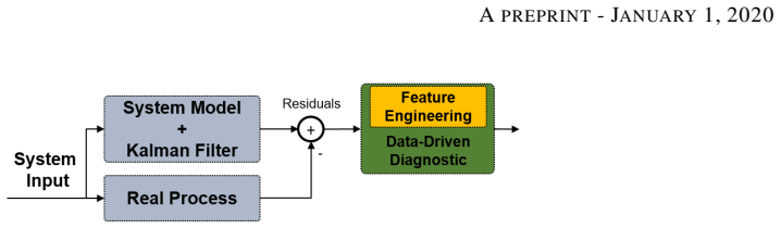
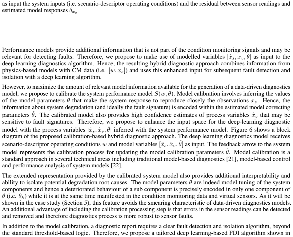
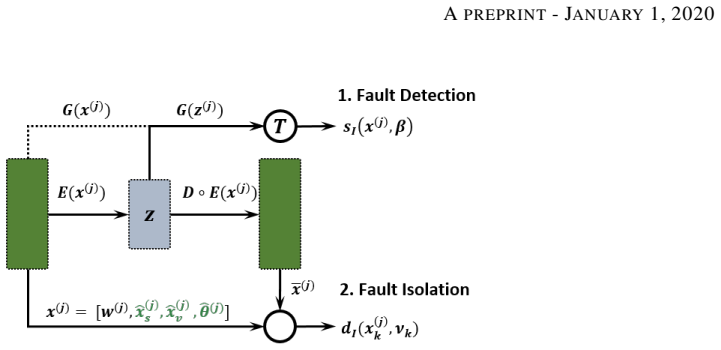
The central mechanism is the calibrated input augmentation: the system model $S(w,\theta)$ is calibrated with an Unscented Kalman Filter to infer the health-parameter vector $\theta$ and the virtual sensors, producing the augmented input $x=[w,\hat{x}_s,\hat{x}_v,\theta]$ that the deep-learning FDI model consumes. The load-bearing property is that each tested fault mode is encoded as a change in one component of $\theta$, so the reconstruction-error isolation score can attribute the fault to a single variable instead of a smeared set of correlated measurements. The same augmented input also feeds the one-class network that performs detection, with a percentile-based threshold on the reconstruction error deciding healthy versus faulty.
What would settle it
Inject a fault that is not captured by any of the ten calibrated health parameters and run the same pipeline; if the isolation step flags an unaffected parameter or reverts to a smeared set of residuals, the central claim of precise isolation is not supported.
Extended reading notes
Core claim
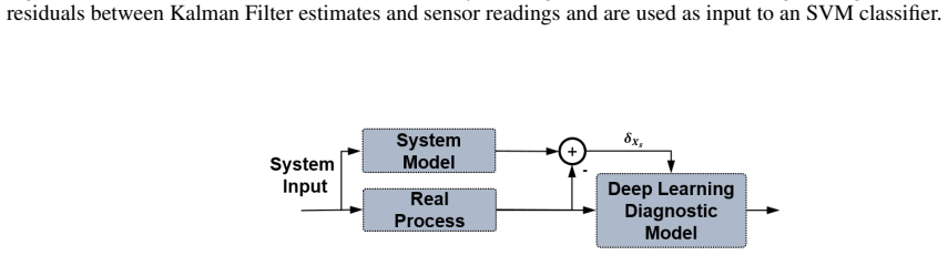
The central claim is that the fault source can be made visible to a learning algorithm by calibrating a system performance model and using the calibrated model's inferred quantities—reconstructed sensor readings, virtual sensors, and component health parameters—as inputs alongside the raw measurements. In the proposed architecture an Unscented Kalman Filter adjusts model parameters so that the model reproduces the observed sensor data; the augmented representation $x=[w,\hat{x}_s,\hat{x}_v,\theta]$ is then fed to an autoencoder-based one-class network for detection and to a reconstruction-similarity index for isolation. The authors report that this calibration-based hybrid input space yields detection accuracies of 97.5 to 100 percent on their simulated C-MAPSS turbofan case, versus 24.5 percent for the best pure data-driven deep model, and that the isolation step flags exactly variable 40, the high-pressure-compressor efficiency modifier, for all four tested faults. They present this precise isolation as removing the smearing effect, in which correlated sensors outside the faulty subsystem also show large reconstruction errors.
Load-bearing premise
The isolation result depends on the real fault being representable as a change in one of the calibrated model parameters that are fed to the network, because the tested faults were injected exactly by changing such a parameter.
Editorial extensions
If this is right
- For systems operated across widely changing conditions, the hybrid calibration-based inputs can turn a one-class deep model into a near-perfect fault detector without requiring any faulty training samples.
- When a fault mode is represented in the model's parameter set, fault isolation can pinpoint the affected component instead of spreading over correlated sensors.
- Detection performance can stay high even when calibration is noisy, because the fault signature also appears in the inferred variables; accurate parameter estimates matter most for isolation rather than detection.
- The framework can be extended by concatenating residuals to the healthy model response with the calibrated variables, which the paper identifies as a natural combined input option.
Reading between the lines
- A natural next test would apply the same calibrated-input recipe to fault modes that are not in the model's parameter list, such as sensor bias or unmodelled wear; the paper itself expects isolation quality to drop in that setting.
- If the pattern transfers, the method could reduce the need for labeled fault data in other safety-critical assets with available performance models, such as power turbines or rotating machinery, though the calibration step would have to be rebuilt for each system.
- The sharp isolation result is partly a consequence of the synthetic setup, where the injected fault is exactly one of the calibrated parameters; a real-world evaluation would need to confirm that the reported single-variable isolation survives model mismatch and sensor noise.
Signed reviews
Editorial analysis
A structured set of objections, weighed in public.
Referee Report
Summary. The paper proposes a hybrid fault detection and isolation framework for complex systems under varying operating conditions. A physics-based performance model is calibrated to measured data with an Unscented Kalman Filter, and the resulting estimates of the measured signals, virtual sensors, and model health parameters are concatenated with the operating conditions to form the input of a one-class autoencoder-based diagnostics model. Fault detection is carried out by a one-class network operating on a latent embedding, and fault isolation is performed by examining per-input reconstruction deviations. The method is evaluated on a synthetic C-MAPSS turbofan dataset with four increasing HPC efficiency degradation faults, and it is compared against feed-forward, AE, VAE, HELM, and OC-SVM baselines with raw, residual, and hybrid inputs. The paper reports near-perfect detection with the hybrid calibrated inputs and states that these inputs isolate only the HPC efficiency parameter, concluding that the physics-enriched inputs outperform pure data-driven approaches and overcome the smearing effect in fault isolation.
Significance. If fully supported, the paper would provide a useful demonstration that adding inferred model states and health parameters to the input space can transform a difficult one-class fault detection problem under transient operating conditions, with the reported detection accuracy rising from roughly 25 percent on raw measurements to near 100 percent on calibrated inputs. The paper is systematic in comparing several deep architectures and includes a noise-robustness analysis of the calibrated features, which is a positive element. However, the evidence for the headline isolation claim is substantially weaker than the abstract suggests: the isolation outcome is largely built into the experimental design, the main experiment uses no sensor noise and no model mismatch, and fault isolation is not scored with a quantitative metric. The contribution is best assessed as a promising architecture and a carefully described case study, not yet as a validated general claim of precise fault isolation.
major comments (3)
- [Section 6.2; Tables 1, 5, and 9] The fault-isolation evaluation is circular with respect to the fault-injection procedure. The four faults are all generated by modifying the HPC efficiency modifier in C-MAPSS (Table 1), the hybrid input includes HPC_eff_mod as variable 40 (Table 5), and the autoencoder flags exactly variable 40 for all four faults (Table 9). Because the same model generates the data and provides the calibration, the isolation result is close to reading out the injected parameter rather than an independent diagnostic inference. This is not an internal inconsistency, but the evaluation does not support the general 'precise isolation' claim in the abstract. The manuscript itself concedes in Sections 7 and 8 that isolation capability will decrease when the calibrated model does not represent the fault mode and leaves faults not represented in the system model to future work. To support the claim, the authors should either evaluate fault modes that are not represented in theta, for example a sensor bias or a fault in a component not captured by the ten modifiers, or explicitly rescope the claim to faults representable in the calibrated parameter set.
- [Section 5.1 and Section 6.2] The validation is conducted in a favorable setting that does not exercise the model-mismatch conditions emphasized in the introduction. No additional sensor noise is used in the main experiment (Section 5.1), and the same C-MAPSS model both generates the condition monitoring data and is used for calibration, so the UKF sees exactly the model class that generated the observations. The robustness experiment in Section 6.1 contaminates the calibration factors after estimation rather than the sensor measurements, and it does not perturb the model structure. The discussion in Section 4.2 acknowledges that model discrepancy, represented as delta(w), remains an open problem. As a result, the paper does not yet demonstrate the claimed benefit 'particularly for systems with a high variability of operating conditions' under realistic mismatch; an experiment with sensor noise, a deliberately misspecified model, or data generated under a different health-parameter evolution would materially strengthen the claim.
- [Section 5.5 and Table 9] Fault isolation is not evaluated with a quantitative metric. Table 9 reports only the indices of variables with dI > 1 for the AE and VAE models, and the text concludes that the hybrid models provide 'perfect isolation,' but there is no measure of isolation accuracy, rank, false-positive rate, or variability across the 10 runs used for detection. Without a defined rule for when isolation is correct and a statistic over runs and fault magnitudes, the reader cannot assess whether variable 40 is flagged overwhelmingly or only marginally above the threshold. Please define an isolation metric, for example the top-1 hit rate for the true parameter or the margin dI_40 minus the maximum dI over the other inputs, and report it with confidence intervals.
minor comments (3)
- [Table 5] Row 45 is assigned the symbol LPT_flow_mod but its description reads 'HPT flow modifier'; this should be corrected to avoid ambiguity with row 43.
- [Section 5.2] The text refers to 'A validation set ST subset DL comprising 6% of the labelled healthy data,' but the training subset was previously also denoted ST and the validation set is SV in Section 4.3 and Figure 9; the notation should be made consistent.
- [Section 5.3] The OC-SVM hyperparameters are selected by maximizing the F1 score on the test set, while the neural-network hyperparameters are selected on the validation set. This oracle choice favors the baseline; the authors should state explicitly that it gives an upper bound on the OC-SVM's realistic performance.
Circularity Check
Isolation to variable 40 is a readout of the injected HPC_eff_mod parameter, so the flagship precision-isolation claim reduces to the fault-injection design.
-
fitted input called prediction
[Section 6.2 (Fault Isolation), with Tables 1, 5, and 9]
"The four faults present in the combined test setsDT+ are rooted in a HPC efficiency deficit. However, not all the models have an input space where the compressor efficiency is represented. Concretely, only the calibration-based hybrid model with inputs [W, ˆXs, ˆXv, ˆθ] has a representation of the HPC efficiency through the estimated model correcting parameters ˆθ. … Finally, hybrid models based on calibrated models with input signals [W, ˆXs, ˆXv, ˆθ] encode the fault signature in only variable 40; which corresponds to the component of θ representing the correction of the HPC efficiency."
The fault mode is defined as HPC efficiency degradation (Table 1), and variable 40 of the hybrid input is HPC_eff_mod (Table 5). The 'perfect isolation' result is therefore the autoencoder flagging the same parameter that was perturbed to create the fault. The UKF-calibrated theta_40 is an input feature, not an independent diagnostic inference; the isolation output is a readout of the fault-injection ground truth. The paper explicitly notes that only the calibrated input has a representation of HPC efficiency, so the result is forced by the experimental design.
-
self definitional
[Section 3.1 (Calibration-Based Hybrid Diagnostics)]
"The model parameters θ are indeed model tuning of the system components and hence a deteriorated behaviour of a sub component is precisely encoded in only one component of θ (i.e. θk) while it is at the same time manifested in the condition monitoring data and virtual sensors. As it will be shown in the case study (Section 5), this feature avoids the smearing characteristic of data-driven diagnostics models."
This asserts as a property of calibration that a sub-component fault is 'precisely encoded' in a single theta component. Combined with the case study's fault definition (HPC efficiency, i.e., theta_40), the promised avoidance of smearing and the later 'perfect isolation' are consequences of the assumed one-to-one fault-to-parameter encoding rather than an empirical discovery.
full rationale
The paper's most distinctive claim is that the hybrid input [W, Xhat_s, Xhat_v, theta] isolates the fault source precisely, overcoming smearing. In the experiment, however, all four faults are the same mode: HPC efficiency degradation (Table 1), and the hybrid input includes the model correcting parameter HPC_eff_mod as variable 40 (Table 5). Section 6.2 states that only the calibrated input has a representation of HPC efficiency and that any such model 'provides perfect isolation' by flagging variable 40. The isolation result is therefore the autoencoder detecting the very parameter that was perturbed to create the fault; it is a calibrated-input readout rather than an independent inference of an unknown root cause. The paper itself acknowledges in Sections 7 and 8 that isolation capability will decrease when the calibrated model does not represent the fault mode, and leaves faults not represented in the system model to future work. This makes the claimed precise isolation conditional on the fault being in theta, i.e., by construction in this evaluation. No self-citation chain or ansatz-smuggling is present; the detection benchmark and network comparisons are self-contained. The score is 6 because the central isolation result reduces to the fault-injection design, while the broader detection comparison retains some independent empirical content.
Assumptions & free parameters
free parameters (5)
- gamma (detection safety margin) =
1.5
- beta (detection threshold) =
P99.9 of validation error times 1.5
- nu_k (per-signal isolation thresholds) =
P99.9 of validation reconstruction error per input component
- OC-SVM hyperparameters =
nu=0.001, gamma=0.1
- Network architecture and training hyperparameters =
one-class [20,100,1]; autoencoder [n,20,8,20,n]; lr 0.001; epochs 500/2000; batch 16/512
assumptions (4)
- domain assumption The C-MAPSS system model is a sufficiently accurate representation of the real physical process (or of the data-generating process).
- ad hoc to paper The fault mode is representable as a change in one calibrated model parameter (HPC_eff_mod).
- domain assumption Test operating conditions are within the distribution of the healthy training set.
- domain assumption The Unscented Kalman Filter yields sufficiently accurate point estimates of theta from the measurements.
Cite this review
Pith. "Pith review of Hybrid deep fault detection and isolation: Combining deep neural networks and system performance models." pith.science (2026). https://pith.science/paper/SMBUGAMF
@misc{pith2026190801529,
  author       = {Pith},
  title        = {Pith review of: Hybrid deep fault detection and isolation: Combining deep neural networks and system performance models},
  year         = {2026},
  howpublished = {\url{https://pith.science/paper/SMBUGAMF}},
  note         = {Machine review of arXiv:1908.01529}
}
read the original abstract
With the increased availability of condition monitoring data and the increased complexity of explicit system physics-based models, the application of data-driven approaches for fault detection and isolation has recently grown. While detection accuracy of such approaches is generally good, their performance on fault isolation often suffers from the fact that fault conditions affect a large portion of the measured signals thereby masking the fault source. To overcome this limitation and enable a more accurate fault detection, we propose a hybrid approach combining physical performance models with deep learning algorithms. Unobserved process variables are inferred with a physics-based performance model to enhance the input space of a data-driven diagnostics model. To validate the effectiveness of the proposed method, we generate a condition monitoring dataset of an advanced gas turbine during flight conditions under healthy and four faulty operative conditions based on the Commercial Modular Aero-Propulsion System Simulation (C-MAPSS) dynamical model. We evaluate the performance of the proposed method in combination with two different deep learning algorithms: feed forward neural networks and Variational Autoencoders, both of which demonstrate a significant improvement when applied within the hybrid fault detection and diagnostics framework. The proposed method is able to outperform pure data-driven solutions, particularly for systems with a high variability of operating conditions. It provides superior results both for fault detection as well as for fault isolation. For fault isolation, it overcomes the smearing effect that is observed in pure data-driven approaches and enables a precise isolation of the affected signal. We also demonstrate that deep learning algorithms provide a better performance on fault detection compared to the traditional machine learning algorithms.
Figures


Figures from the paper (17 more)





Reference graph
Works this paper leans on
-
[1]
Deep Learning and Its Applications to Machine Health Monitoring: A Survey
Rui Zhao, Ruqiang Yan, Zhenghua Chen, Kezhi Mao, Peng Wang, and Robert X Gao. Deep Learning and Its Applications to Machine Health Monitoring: A Survey. Technical report, dec 2016
work page 2016
-
[2]
A review on the application of deep learning in system health management, jul 2018
Samir Khan and Takehisa Yairi. A review on the application of deep learning in system health management, jul 2018
work page 2018
-
[3]
Online class imbalance learning and its applications in fault detection
Shuo Wang, Leandro L Minku, and Xin Yao. Online class imbalance learning and its applications in fault detection. International Journal of Computational Intelligence and Applications, 12(04):1340001, 2013
work page 2013
-
[4]
Le Xu, Mo-Yuen Chow, and Leroy S Taylor. Power distribution fault cause identification with imbalanced data using the data mining-based fuzzy classificatione-algorithm. IEEE Transactions on Power Systems, 22(1):164–171, 2007
work page 2007
-
[5]
Yuyan Zhang, Xinyu Li, Liang Gao, Lihui Wang, and Long Wen. Imbalanced data fault diagnosis of rotating machinery using synthetic oversampling and feature learning. Journal of manufacturing systems, 48:34–50, 2018
work page 2018
-
[6]
Piero Baraldi, Francesco Di Maio, Pietro Turati, and Enrico Zio. Robust signal reconstruction for condition monitoring of industrial components via a modified auto associative kernel regression method. Mechanical Systems and Signal Processing, 60:29–44, 2015
work page 2015
-
[7]
Fault detection based on signal reconstruction with auto-associative extreme learning machines
Yang Hu, Thomas Palmé, and Olga Fink. Fault detection based on signal reconstruction with auto-associative extreme learning machines. Engineering Applications of Artificial Intelligence, 57:105–117, 2017
work page 2017
-
[8]
Deep feature learning network for fault detection and isolation
Gabriel Michau, Thomas Palmé, and Olga Fink. Deep feature learning network for fault detection and isolation. In PHM 2017, St. Petersburg, USA, 2-5 October 2017, pages 108–118. PHM Society, 2017
work page 2017
Show all 35 references
-
[9]
Domain adaptive transfer learning for fault diagnosis
Qin Wang, Gabriel Michau, and Olga Fink. Domain adaptive transfer learning for fault diagnosis. arXiv preprint arXiv:1905.06004, 2019
1905 arXiv
-
[10]
User’s Guide for the Commercial Modular Aero-Propulsion System Simulation (C-MAPSS)
Dean K Frederick, Jonathan A Decastro, and Jonathan S Litt. User’s Guide for the Commercial Modular Aero-Propulsion System Simulation (C-MAPSS). Technical report, 2007
2007
-
[11]
DASHlink - Flight Data For Tail 687, 2012
2012
-
[12]
Support vector method for novelty detection
Bernhard Schölkopf, Robert Williamson, Alex Smola, John Shawe-Taylor, and John Piatt. Support vector method for novelty detection. In Advances in Neural Information Processing Systems, pages 582–588, 2000
2000
-
[13]
Hybrid Model-Based and Data-Driven Fault Detection and Diagnostics for Commercial Buildings
Stephen Frank, Mike Heaney, Xin Jin, Joseph Robertson, Howard Cheung, Ryan Elmore, and Gregor P Henze. Hybrid Model-Based and Data-Driven Fault Detection and Diagnostics for Commercial Buildings. Proceedings of the ACEEE Summer Study on Energy Efficiency in Buildings, Aug 21-26...
2016
-
[14]
Hybrid Physics-Based and Data-Driven Phm
H Hanachi, W Yu, I Y Kim, and C K Mechefske. Hybrid Physics-Based and Data-Driven Phm. In Canadian Machinery Vibration Association (CMVA) Annual Conference, Edmonton, Alberta, Canada, 2017
2017
-
[15]
Rausch, Kai F
Randal T. Rausch, Kai F. Goebel, Neil H. Eklund, and Brent J. Brunell. Integrated In-Flight Fault Detection and Accommodation: A Model-Based Study. In Volume 1: Turbo Expo 2005, pages 561–569. ASME, 2005
2005
-
[16]
Variations on the Kalman Filter for Enhanced Performance Monitoring of Gas Turbine Engines
S.J Borguet. Variations on the Kalman Filter for Enhanced Performance Monitoring of Gas Turbine Engines. Phd thesis, Université de Liège, 2012
2012
-
[17]
Physics Guided Recurrent Neural Networks For Modeling Dynamical Systems: Application to Monitoring Water Temperature And Quality In Lakes
Xiaowei Jia, Anuj Karpatne, Jared Willard, Michael Steinbach, Jordan Read, Paul C Hanson, Hilary A Dugan, and Vipin Kumar. Physics Guided Recurrent Neural Networks For Modeling Dynamical Systems: Application to Monitoring Water Temperature And Quality In Lakes. Technical repor...
2018
-
[18]
Renato Giorgiani Nascimento and Felipe A.C. Viana. Fleet prognosis with physics-informed recurrent neural networks. In Structural Health Monitoring 2019: Enabling Intelligent Life-Cycle Health Management for Industry Internet of Things (IIOT) - Proceedings of the 12th Internat...
2019
-
[19]
Arinan Dourado and Felipe A. C. Viana. Physics-Informed Neural Networks for Corrosion-Fatigue Prognosis. Proceedings of the Annual Conference of the PHM Society, 11(1), sep 2019
2019
-
[20]
Wind Turbine Main Bearing Fatigue Life Estimation with Physics- informed Neural Networks
Yigit Anil Yucesan and Felipe A C Viana. Wind Turbine Main Bearing Fatigue Life Estimation with Physics- informed Neural Networks. In Phm 2019, volume 11, pages 1–14, 2019
2019
-
[21]
Brent J.; Brunell, Jr. Harry K. Mathews, and Aditya Kumar. United States Patent Design of an Adaptive Model-Based Control for Controlling a Gas Turbine, 2004
2004
-
[22]
Lilley, Peter Mathé, and V olker Schloßhauer
Manuel Arias Chao, Darrel S. Lilley, Peter Mathé, and V olker Schloßhauer. Calibration and Uncertainty Quan- tification of Gas Turbine Performance Models. In Proceedings of the ASME Turbo Expo , volume 7A, page V07AT29A001, 2015
2015
-
[23]
W. J. Scheirer, A. de Rezende Rocha, A. Sapkota, and T. E. Boult. Toward Open Set Recognition. IEEE Transactions on Pattern Analysis and Machine Intelligence, 35(7):1757–1772, 2013
2013
-
[24]
New extension of the Kalman filter to nonlinear systems
Simon J Julier and Jeffrey K Uhlmann. New extension of the Kalman filter to nonlinear systems. In Signal Processing, Sensor Fusion, and Target Recognition VI, volume 3068, page 182, 1997
1997
-
[25]
Moya and Don R
Mary M. Moya and Don R. Hush. Network constraints and multi-objective optimization for one-class classification. Neural Networks, 9(3):463–474, 1996
1996
-
[26]
Feature Learning for Fault Detection in High- Dimensional Condition-Monitoring Signals
Gabriel Michau, Yang Hu, Thomas Palmé, and Olga Fink. Feature Learning for Fault Detection in High- Dimensional Condition-Monitoring Signals. Submitted for a possible publication in IEEE Transactions on Cybenetics, 2017
2017
-
[27]
Hierarchical Extreme Learning Machine for unsupervised representation learning
Wentao Zhu, Jun Miao, Laiyun Qing, and Guang-Bin Huang. Hierarchical Extreme Learning Machine for unsupervised representation learning. In 2015 International Joint Conference on Neural Networks (IJCNN), pages 1–8. IEEE, 2015
2015
-
[28]
Auto-encoding variational bayes
Diederik P Kingma and Max Welling. Auto-encoding variational bayes. In 2nd International Conference on Learning Representations, ICLR 2014 - Conference Track Proceedings, 2014
2014
-
[29]
Pedregosa, G
F. Pedregosa, G. Varoquaux, A. Gramfort, V . Michel, B. Thirion, O. Grisel, M. Blondel, P. Prettenhofer, R. Weiss, V . Dubourg, J. Vanderplas, A. Passos, D. Cournapeau, M. Brucher, M. Perrot, and E. Duchesnay. Scikit-learn: Machine learning in Python. Journal of Machine Learni...
2011
-
[30]
Adam: A method for stochastic optimization
Diederik P Kingma and Jimmy Lei Ba. Adam: A method for stochastic optimization. In 3rd International Conference on Learning Representations, ICLR 2015 - Conference Track Proceedings, 2015
2015
-
[31]
Understanding the difficulty of training deep feedforward neural networks
Xavier Glorot and Yoshua Bengio. Understanding the difficulty of training deep feedforward neural networks. Technical report, 2010
2010
-
[32]
LeCun, Léon Bottou, Genevieve B
Yann A. LeCun, Léon Bottou, Genevieve B. Orr, and Klaus Robert Müller. Efficient backprop. Lecture Notes in Computer Science (including subseries Lecture Notes in Artificial Intelligence and Lecture Notes in Bioinformatics), 7700 LECTU:9–48, 2012
2012
-
[33]
Hands-on transfer learning with Python : implement advanced deep learning and neural network models using TensorFlow and Keras
Dipanjan Sarkar, Raghav Bali, and Tamoghna Ghosh. Hands-on transfer learning with Python : implement advanced deep learning and neural network models using TensorFlow and Keras. 2018
2018
-
[34]
InfoV AE: Balancing Learning and Inference in Variational Autoencoders
Shengjia Zhao, Jiaming Song, and Stefano Ermon. InfoV AE: Balancing Learning and Inference in Variational Autoencoders. In Proceedings of the AAAI Conference on Artificial Intelligence, volume 33, pages 5885–5892, jul 2019
2019
-
[35]
Tutorial on Variational Autoencoders
Carl Doersch. Tutorial on Variational Autoencoders. Technical report, jun 2016. 21 A PREPRINT - JANUARY 1, 2020 Figure 18: Simplified diagram of the turbo fan engine model in C-MAPSS with Fan, Combustor, High-pressure compressor (HPC); high-pressure turbine (HPT); Low-pressure ...
2016
Reviewed August 14, 2026 · model on record in the stance chip above.
Discussion (0). Continue with ORCID to comment.