REVIEW 3 major objections 5 minor 33 references
Effect of rotation and magnetic field in the gyroscopic precession around a neutron star
T0 review · 3 major / 5 minor · reviewed 2026-08-14 · deepseek-v4-flash
Pith's one-line read The precession of a test gyroscope encodes a neutron star's mass, rotation, and magnetic-field configuration, and the pattern distinguishes neutron stars from black holes.
desk verdict A correct forward calculation of gyro precession in numerical NS spacetimes, but the BH/NS comparison and interior null points rest on arbitrary non-geodesic orbits; the astrophysical interpretation needs a geodesic-Ω rerun. read the letter →
The pith
A machine-rendered reading of the paper's core claim, the machinery that carries it, and where it could break.
The reading
What carries the argument
The load-bearing object is the timelike Killing vector $K=\partial_t+\Omega\partial_\varphi$, a symmetry direction of the stationary, axisymmetric spacetime, together with the spin-precession formula $\tilde{\Omega}_P = \frac{1}{2K^2}(\tilde{K}\wedge d\tilde{K})$. This combines geodetic precession from spacetime curvature with frame-dragging from rotation and magnetic fields. In the conformally flat XNS metric the formula reduces to an explicit expression (Eq. 13) for the precession vector in terms of the lapse $\alpha$, shift $\beta^\varphi$, and conformal factor $\psi$, using the metric coefficients supplied by the XNS code. The timelike condition $K^2<0$ sets the allowed range of $\Omega$ at every radius and angle. Inside the star the frame-dragging term $d g_{t\varphi}/dr$ and the orbital term $\Omega\, d g_{\varphi\varphi}/dr$ compete and produce the null points that carry the paper's signatures.
What would settle it
Recompute the precession curves using geodesic circular-orbit frequencies $\Omega_{\rm geo}(r)$ derived from the same XNS metric; if the interior null point and the finite-inside-the-star pattern disappear, the identification with real particles fails. Observationally, measure the precession of accreting clumps around a known neutron star and check whether the null point appears at the predicted radius.
Extended reading notes
Core claim
The central claim is that the overall gyroscope precession frequency $\Omega_P$, computed from the Killing-vector formula $\tilde{\Omega}_P = \frac{1}{2K^2}(\tilde{K}\wedge d\tilde{K})$ with $K=\partial_t+\Omega\partial_\varphi$, is a faithful probe of strong-gravity spacetimes. For a neutron star modeled by the XNS code with a polytropic equation of state, $|\Omega_P|$ is finite everywhere, has an interior local minimum (a null point) along the equatorial plane, and asymptotes to the gyroscope's orbital frequency far from the star. For a Kerr black hole, the same quantity diverges as the gyroscope approaches the ergosphere. The paper further claims that the shape and null-point locations of the $\Omega_P(r)$ curves respond systematically to the star's mass, spin, magnetic-field strength, and field configuration, so the gyro frequency can distinguish a black hole from a neutron star and can separate poloidal from toroidal magnetic-field distributions.
Load-bearing premise
The calculation assumes that assigning the gyroscope any angular velocity at which an observer would move slower than light produces a worldline a real particle could follow, but it never checks whether those circular orbits satisfy the geodesic (free-fall) equation.
Editorial extensions
If this is right
- A measured gyro precession curve near a compact object can identify the object: divergence at the ergosphere marks a black hole, while a finite interior curve with a null point marks a neutron star.
- The location of the null point shifts with the gyroscope's orbital frequency and with the star's spin, so timing precession of accreting matter could constrain both the star's rotation rate and the orbital dynamics of the accretion disk.
- Poloidal and toroidal magnetic fields leave opposite imprints on the interior precession curve: stiffer with a deeper minimum for poloidal fields, flatter with no minimum for toroidal fields, so the curve can reveal which field geometry dominates in magnetars.
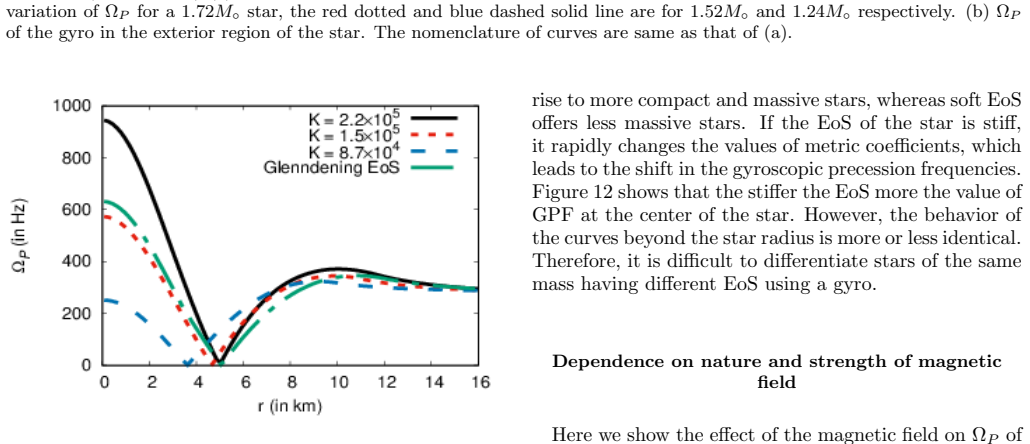
- Because the precession frequency depends on the star's mass and equation of state, precise precession measurements could help pin down neutron-star masses and, indirectly, the equation of state; the paper notes exterior curves are less discriminating for equal-mass stars.
Reading between the lines
- A self-consistency check would recompute the curves using geodesic circular orbits whose orbital frequency is derived from the same metric; if the interior null point survives the geodesic constraint, the identification of the gyro with real accreting particles is on firmer ground.
- The same Killing-vector precession machinery could be applied to other stationary axisymmetric neutron-star models, such as stars with anisotropic pressure or exotic equations of state, to test whether the finite-inside-the-star signature and the black-hole divergence are generic.
- If quasi-periodic oscillations in X-ray binaries are driven by precession, the predicted null-point radii could be compared with observed QPO frequencies, giving an observational route to test the paper's interpretation.
Signed reviews
Editorial analysis
A structured set of objections, weighed in public.
Referee Report
Summary. The paper studies the general-relativistic spin precession of a test gyroscope moving on circular orbits with a prescribed constant angular velocity around neutron stars. It derives a precession-frequency formula from the standard Killing-vector expression, uses the XNS code to model rotating and magnetized neutron stars, and examines the dependence of the precession frequency on the gyro's orbital angular velocity, the stellar rotation rate, mass, equation of state, and poloidal versus toroidal magnetic field configurations. It also compares the result with the Kerr black-hole case, and claims that the precession frequency can be used to distinguish black holes from neutron stars and to probe neutron-star mass and magnetic-field structure.
Significance. If the calculations describe real particles, the paper would offer a potentially useful probe of neutron-star mass and magnetic-field geometry, and a new way to contrast black holes and neutron stars. The formal derivation from Eq. (1) is standard, and the Schwarzschild-limit comparison in Fig. 4 is a genuine validation of the numerical setup. The calculation is forward and transparent, with no fitting to observational data, and the free parameters are clearly identified. However, the astrophysical interpretation is undermined by the use of non-geodesic, hand-picked orbital frequencies, and the numerical results are presented without convergence checks or error estimates. The central claims are therefore not yet established for physical particles.
major comments (3)
- [Sec. II, Eqs. (2), (28); Sec. IV, Figs. 6–8] The gyroscope worldlines are integral curves of K = ∂_t + Ω∂_φ with Ω chosen by hand (100–500 Hz) subject only to the timelike condition K² < 0, Eq. (28). For a free circular orbit, Ω is not a free parameter but is fixed by the geodesic condition, e.g., d/dr[g_tt + 2Ωg_tφ + Ω²g_φφ] = 0 in the equatorial plane. This condition is never imposed. Consequently, the claimed black-hole/neutron-star distinction is not established: the divergence in Fig. 6(a) near the ergosphere for Ω = 500 Hz is a property of this family of forced observers, since a 500 Hz free circular orbit around a 1.5 M☉ object lies near r ≈ 27 km, far from the ergosphere at r ≈ 4.4 km. Likewise, the interior null points in Figs. 7 and 8 describe forced observers inside the star rather than accretion-disk particles. The Introduction and Section V explicitly interpret the gyro as representing real particles in the star or accretion disk, and Section V's closing sentence restricts the gyros to particles encircling the NS; these interpretations are mutually inconsistent without the geodesic condition. I request either a recomputation for geodesic circular orbits, with Ω_geo(r) solved from the effective potential, or a substantial retraction of the physical particle claims in favor of statements about prescribed circular observers.
- [Sec. IV, Figs. 4, 13, 14] The numerical results are reported without any convergence tests or error estimates. The static XNS result in Fig. 4 is described as matching the Schwarzschild configuration 'reasonably', but no quantitative deviation is given. The magnetic-field effects in Figs. 13 and 14 are differences between curves at the same radius, and without an estimate of numerical error it is not possible to judge whether the claimed poloidal/toroidal distinctions are significant. Please provide convergence tests with respect to XNS grid resolution and a quantitative comparison in Fig. 4, and include error estimates or at least a statement of the numerical uncertainty in the plotted quantities.
- [Sec. IV, subsection 'Dependence on the angular velocity of the NS'] The statement that the gyro precession 'goes to zero at the center of the star' whenever the gyro angular velocity equals the stellar angular velocity is claimed to be robust, but no analytic proof is given. Equation (13) shows that the central value depends on metric derivatives at r = 0 in the specific XNS coordinates, and the regularity of those derivatives is not demonstrated. If this is intended as a general result, it should be proved from Eq. (13) under the stated symmetry assumptions; otherwise, it should be presented as a property of the particular numerical solution, with a check that it is not a coordinate artifact.
minor comments (5)
- [Sec. I and Sec. II] The name 'Lense-Thirring' is misspelled as 'lense and thrilling' and 'lense thrilling'; please correct these to 'Lense and Thirring' and 'Lense-Thirring'.
- [Figs. 6–12] The solar mass is denoted variously as 'M0' and 'M◦'; please use a consistent symbol such as M_☉.
- [Fig. 5 caption] The caption identifies the 'green solid-dashed curve' twice as prograde motion; one of these should presumably be retrograde motion.
- [Sec. III, Eq. (17)] The polytropic constant K and its quoted values (e.g., K = 1.5 × 10^5) are given without units; please specify the cgs units used.
- [Sec. II, Eq. (12)] The term 'Copernican basis' is nonstandard; please identify the orthonormal tetrad explicitly and define how the 'overall' magnitude |Ω_P| is computed.
Circularity Check
No significant circularity: the gyro precession is computed forward from an assumed metric and field configuration, with no fitted target data or self-citation chain.
full rationale
The derivation is self-contained and forward. Eq. (13) is the standard spin-precession formula for a gyroscope carried along integral curves of the Killing vector K = ∂t + Ω∂φ (Eq. 2), and the metric coefficients are obtained by solving the XNS Einstein equations with assumed EoS and magnetic-field distributions. The paper validates the code against the static Schwarzschild limit (Fig. 4), providing an independent check. No parameter is fitted to any target observable, and no output quantity is reused as an input: the mass, rotation rate, magnetic-field strength/geometry, and gyro orbital frequency Ω are all free inputs, and the GPF is evaluated once. The BH/NS comparison is a forward calculation in two different spacetimes (Kerr vs. XNS), not a fit. The paper's citations [25]-[31] are to Chakraborty et al. and other groups, not to the present authors, and the quoted precession formula is a standard GR result, not an unverified uniqueness claim. The main physical weakness, that the chosen Ω is not required to satisfy the geodesic condition, so some plotted worldlines are forced observers rather than free accretion-disk particles, is a correctness and interpretation risk rather than a circularity: it does not make the calculated precession equal to an input by construction. Accordingly there are no circular steps and the score is 0.
Assumptions & free parameters
free parameters (4)
- Orbital angular velocity Ω of the gyroscope =
100, 200, 500 Hz (varied by hand)
- Polytropic EoS constant K =
1.5e5, 2.2e5, 8.7e4 (cgs style units), plus tabulated Glendenning
- Central energy density =
1.2e15 g cm^-3; also 5.1e14 g cm^-3 in Fig. 5
- Central magnetic field strength =
poloidal up to 1e18 G; toroidal up to 8e17 G
assumptions (7)
- domain assumption Spacetime is stationary and axisymmetric
- domain assumption Test gyroscope has zero mass and does not back-react on the spacetime
- domain assumption Gyroscope worldline is an orbit of the Killing vector K = ∂t + Ω∂φ
- domain assumption Conformal flatness of the spatial metric
- domain assumption Magnetic field distribution is poloidal or toroidal with specified central strengths
- domain assumption Polytropic EoS with γ=2 and chosen K describes the neutron-star matter
- standard math Standard spin precession formula ΩP = (1/(2K^2)) ⋆(K ∧ dK)
Cite this review
Pith. "Pith review of Effect of rotation and magnetic field in the gyroscopic precession around a neutron star." pith.science (2026). https://pith.science/paper/SRGETAVX
@misc{pith2026190803889,
  author       = {Pith},
  title        = {Pith review of: Effect of rotation and magnetic field in the gyroscopic precession around a neutron star},
  year         = {2026},
  howpublished = {\url{https://pith.science/paper/SRGETAVX}},
  note         = {Machine review of arXiv:1908.03889}
}
read the original abstract
We study the overall spin precession frequency of a test gyroscope around a neutron star. The precession of the test gyroscope gives the signatures of the general relativistic effects that are present in the region of strong gravity of an NS. Using a numerical code, we find the precession of the test gyroscope for a rotating and a strongly magnetized neutron star. The magnetic field distribution inside the neutron star is assumed either to be poloidal or toroidal. The overall spin precession rate is obtained by setting the orbital frequency of the gyroscope to a non-zero value but restricted to a time-like observer. The gyro frequency differs depending on the central object being a black hole or a neutron star. For neutron star, the gyro precession can even be calculated inside the star. We find that the gyroscope precession frequency depends on the stars mass, rotation rate, and magnetic field configuration.
Figures


Figures from the paper (8 more)




Reference graph
Works this paper leans on
-
[1]
B. P. Abbott et al., Phys. Rev. Lett. 116, 061102 (2016)
2016
-
[2]
B. P. Abbott et al., Phys. Rev. Lett. 119, 161101 (2017)
2017
- [3]
-
[4]
Margalit and B
B. Margalit and B. D. Metzger, Astrophys. J. Lett. 850, L19 (2017)
2017
-
[5]
Radice, Astrophys
D. Radice, Astrophys. J. Lett. 838, L2 (2017)
2017
-
[6]
M. Ruiz, S. L. Shapiro, and A. Tsokaros, Phys. Rev. D 97, 021501 (2018)
2018
-
[7]
The angular velocity of the gyroscope is positive with respect to the angular velocity of the star (prograde mo- 8 FIG. 9. (Color online)(a) ΩP of gyro along different azimuthal positions around a 1.5M◦ NS (ω = 700Hz) with positive or- bital angular velocity Ω = 100Hz. The black solid curve, red dotted curve and blue dashed curve are for θ = 0 ◦, 45◦, 90◦ ...
-
[8]
Shibata, S
M. Shibata, S. Fujibayashi, K. Hotokezaka, K. Kiuchi, K. Kyutoku, Y. Sekiguchi, and M. Tanaka, Phys. Rev. D 96, 123012 (2017)
2017
Show all 33 references
-
[9]
E. R. Most, L. R. Weih, L. Rezzolla, and J. Schaffner- Bielich, Phys. Rev. Lett. 120, 261103 (2018)
2018
-
[10]
Demorest, T
P. Demorest, T. Pennucci, S. Ransom, M. Roberts, and J. Hessels, Nature (London) 467, 1081 (2010)
2010
-
[11]
Antonidis, P
J. Antonidis, P. C. C. Freire, N. Wex et al., Science 340, 1233232 (2013)
2013
-
[12]
R. C. Duncan and C. Thompson, AstroPhys. J. 392, L9 (1992)
1992
-
[13]
Thompson and R
C. Thompson and R. C. Duncan, AstroPhys. J. 408, 194 (1993)
1993
-
[14]
Mereghetti and L
S. Mereghetti and L. Stella, Astrophys. J. 442, L17 (1995)
1995
-
[15]
Baykal, A., & Swank, J., Astrophys. J. 460, 470 (1996)
1996
-
[16]
H., Strohmayer, T., & Stark, M
Baykal, A., Swank, J. H., Strohmayer, T., & Stark, M. J., Astron. & Astrophys. 336, 173 (1998)
1998
-
[17]
Kouveliotou et al., Nature 393, 235 (1998)
C. Kouveliotou et al., Nature 393, 235 (1998)
1998
-
[18]
S. R. Kulkarni and D. A. Frail, Nature 365, 33 (1993)
1993
-
[19]
Murakami et al., Nature 368, 127 (1994)
T. Murakami et al., Nature 368, 127 (1994)
1994
-
[20]
Chatterjee, C
D. Chatterjee, C. Chakraborty and D. Bandyopadhyay, JCAP 1701 (2017) no.01, 062
2017
-
[21]
Lense and H
J. Lense and H. Thirring, Phys. Z. 19, (1918) 156
1918
-
[22]
B., ApJ, 150, 1005 (1967)
Hartle, J. B., ApJ, 150, 1005 (1967)
1967
-
[23]
K., & Weber, F
Glendenning, N. K., & Weber, F. 1994, PhRvD, 50, 3836
1994
-
[24]
M., & Stella, L
Morsink, S. M., & Stella, L. 1999, ApJ, 513, 827
1999
-
[25]
1999, Pulsars as Astrophysical Laboratories for Nuclear and Particle Physics (Bristol: IOP Publishing)
Weber, F. 1999, Pulsars as Astrophysical Laboratories for Nuclear and Particle Physics (Bristol: IOP Publishing)
1999
-
[26]
Chakraborty, K
C. Chakraborty, K. P. Modak and D. Bandyopadhyay, Astrophys. J. 790 (2014) no.1, 2
2014
-
[27]
N Straumann, General Relativity with Applications to Astrophysics, 2009, Springer
2009
-
[28]
Chakraborty, M
C. Chakraborty, M. Patil, P. Kocherlakota, S. Bhat- tacharyya, P. S. Joshi and A. Krlak, Phys. Rev. D 95 (2017) no.8, 084024
2017
-
[29]
Bucciantini, N., Del Zanna, L, General relativistic mag- netohydrodynamics in axisymmetric dynamical space- times: the X-ECHO code, Astronomy and Astrophysics 528, A101 (2011)
2011
-
[30]
Hidemi Komatsu, Yoshiharu Eriguchi, Izumi Hachisu, MNRAS 237, 355 (1989)
1989
-
[31]
Chakraborty, Eur
C. Chakraborty, Eur. Phys. J. C 75 (2015) no.12, 572
2015
-
[32]
Chakraborty and P
C. Chakraborty and P. Majumdar, Class. Quant. Grav. 31 (2014) 075006
2014
-
[33]
N. K. Glendenning and S. A. Moszkowski, Phys. Rev. Lett. 67, 2414 (1991)
1991
Reviewed August 14, 2026 · model on record in the stance chip above.
Discussion (0). Continue with ORCID to comment.