REVIEW 3 major objections 7 minor 46 references
Numerical comparison of energy- versus circulation-preserving stochastic vortex dynamics
T0 review · 3 major / 7 minor · reviewed 2026-08-02 · deepseek-v4-flash
Pith's one-line read Choosing which invariant to preserve — circulation or kinetic energy — determines whether stochastic uncertainty in 2D vortex flows concentrates at sharp gradients or spreads across the domain.
desk verdict Useful first systematic SALT-vs-SFLT comparison for 2D vortex flows, but the headline |k|^2 scaling is an artifact of the noise normalization in Eq. (33), not an intrinsic property. read the letter →
The pith
A machine-rendered reading of the paper's core claim, the machinery that carries it, and where it could break.
The reading
What carries the argument
The central object is the comparison of the two stochastic interaction terms in the Lie–Poisson formulation. In spectral space, the SALT bracket {F_m, ω_k} scales as |k|² times the SFLT bracket {ψ_k, F_m}, because vorticity is the Laplacian of the stream function and therefore carries amplified high-wavenumber content. In physical space, the analogous object is the gradient ratio ∂ω/∂r ÷ ∂ψ/∂r = 4c(cr²−2) for a Gaussian vortex, which grows with the sharpness parameter c. This ratio is the mechanism that converts the conservation choice into a scale-sensitivity and localization statement.
What would settle it
Run the traveling dipole and vortex-merger experiments with the SFLT amplitude θ_k scaled by a wavenumber-independent factor different from 4π². If the ratio of SALT-induced to SFLT-induced variance no longer grows like |k|², the claimed scaling is an artifact of calibration rather than intrinsic. Alternatively, compute the power spectrum of the ensemble variance field: SALT variance should dominate at high wavenumbers and SFLT at low wavenumbers for the same noise basis.
Extended reading notes
Core claim
The paper shows that the abstract choice of which geometric invariant to preserve has a concrete, measurable consequence. In spectral space, the SALT term {F_m, ω_k} carries a prefactor 16π⁴|k|² while the SFLT term {ψ_k, F_m} carries 4π², so the same Fourier mode excites flow components a factor |k|² more strongly when added as transport noise than when added as forcing noise. In physical space, an idealized Gaussian vortex gives the same message through the ratio of vorticity to stream-function gradients, 4c(cr²−2), which grows as vortices shrink. The numerical ensembles confirm that SALT localizes uncertainty along active vorticity gradients and SFLT distributes it globally. The authors de
Load-bearing premise
The quantitative comparison depends on the noise calibration θ_k = σ 4π² F_k chosen to 'ensure a fair comparison' (Eq. 33); with a different relative amplitude between SALT and SFLT forcings, the |k|² ratio and the degree of localization would change.
Editorial extensions
If this is right
- Circulation-preserving SALT places ensemble uncertainty exactly where vorticity gradients are strong; energy-preserving SFLT spreads it broadly, so the two frameworks answer different uncertainty-quantification questions.
- Because SALT's noise grows with wavenumber, uncalibrated SALT amplitude can artificially accelerate small-vortex break-up; SFLT is less prone to this when the location of coherent structures is not well known.
- The mean-field versions LA SALT and EA SFLT inherit the contrast: LA SALT's diffusive term is driven by expected vorticity (sharp), EA SFLT's by expected stream function (smooth), so their regularization also differs in locality.
- Since simultaneously preserving both energy and circulation reduces the noise to a stochastic time reparametrization, modelers must choose one invariant; the paper demonstrates that the choice has observable consequences for forecast spread.
Reading between the lines
- A direct test of the mechanism: measuring the wavenumber spectrum of the ensemble variance field in a homogeneous turbulent run should show SALT variance concentrated at higher wavenumbers than SFLT variance at the same noise amplitude.
- The claimed |k|² ratio is calibrated by the specific normalization θ_k = σ 4π² F_k; if a different relative amplitude were chosen, the absolute ratio would change, though the qualitative localization contrast may persist.
- If the gradient-ratio mechanism is generic, the same localization-versus-spreading contrast should appear in shallow-water and MHD extensions that the paper proposes; these are natural settings to test it.
- The paper explicitly defers the turbulent-regime comparison of the averaged frameworks LA SALT and EA SFLT; testing whether their regularization difference survives in forced turbulence is a clear next step.
Editorial analysis
A structured set of objections, weighed in public.
Referee Report
Summary. The paper compares two geometric stochastic frameworks for the 2D incompressible Euler equations: SALT (circulation-preserving, via stochastic advection by Lie transport) and SFLT (energy-preserving, via stochastic forcing by Lie transport), together with their averaged variants LA SALT and EA SFLT. In §3.1 the authors derive a spectral comparison of the two noise terms, obtaining a ratio proportional to ||k||^2, which they interpret as SALT being more sensitive to high-frequency flow components and acting as a localized perturbation, whereas SFLT is a more regularized global forcing. This interpretation is tested numerically in three setups: a traveling dipole, vortex merger, and forced-damped turbulence. The numerical results show that SALT produces variance concentrated near vorticity gradients, while SFLT produces a more diffuse variance field. The paper concludes that the choice of geometric invariant determines the scale sensitivity and spatial distribution of modeled uncertainty.
Significance. If the central claim holds, the paper would provide practically useful guidance for selecting between circulation-preserving and energy-preserving stochastic parameterizations in geophysical fluid dynamics, a question of current interest. The manuscript has clear strengths: the derivations of the bracket identities are explicit and self-contained; no empirical constants are fitted; the numerical implementation uses the open-source Firedrake package and is described in enough detail to be reproducible; and the prediction that SALT localizes uncertainty near vorticity gradients is falsifiable. However, the headline quantitative claim—the ||k||^2 scaling of SALT relative to SFLT—is conditional on an ad-hoc normalization in Eq. (33). The numerical experiments inherit that normalization, so they cannot independently validate the scaling. The significance of the paper is therefore real but lower than the abstract suggests, and the qualitative localization contrast, while plausible, needs to be disentangled from the chosen calibration.
major comments (3)
- [§3.1 and §4.2, Eqs. (23)–(24) and (32)–(33)] The central claim that 'noise effects scale by |k|^2 relative to SFLT' is not an intrinsic property of the two frameworks; it is determined by the arbitrary normalization θ_k = σ4π²F_k in Eq. (33). The spectral comparison gives a ratio 4π²||k||² between the SALT bracket {F_m, ω_k} and the SFLT bracket {ψ_k, F_m}. If the SFLT scalar is written θ_k = αF_k, the actual SFLT noise amplitude for that mode becomes α{ψ_k, F_m}, and the ratio becomes 4π²||k||²/α. Equation (33) sets α=4π², which converts the ratio to exactly ||k||². No physical or statistical principle is provided for this choice. Setting α=4π²||k||² (so that the SFLT forcing is the vorticity of the SALT noise velocity) would make the ratio 1, eliminating the claimed scale-sensitivity. The numerical experiments use this same normalization and thus cannot independently validate the scaling; they illustrate the consequences of Eq. (
- [§3.1, Eqs. (23)–(24)] The spectral comparison is local in state space and does not by itself establish the relative magnitude of noise effects in the stochastic dynamics. It compares the magnitudes of the noise vector fields {F_m, ω_k} and {ψ_k, F_m} for a single Fourier mode of the current state, but the actual effect on the ensemble variance is governed by the full nonlinear SPDEs (12) and (15), including the Itô correction and the coupled time evolution of ψ and ω. The claimed 'scaling by |k|^2' is therefore a heuristic indicator, not a proven property of the two frameworks. Because the numerical tests inherit the normalization of Eq. (33), they cannot resolve this gap. I recommend either deriving the variance/covariance dynamics in Fourier space (e.g., from the LA SALT/EA SFLT expectation equations) or softening the wording in the Abstract and §5 so that the scaling is presented as a conditional observati
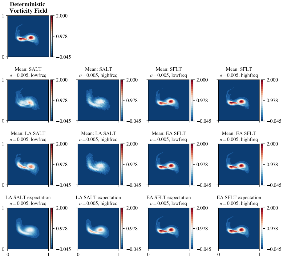
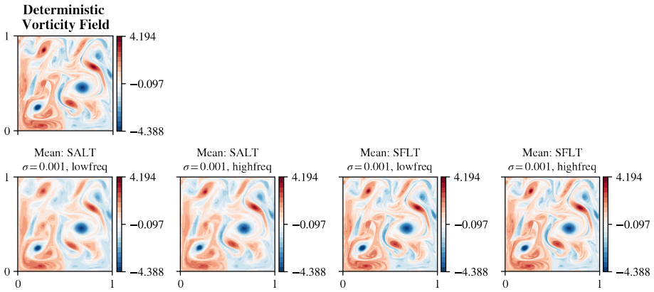
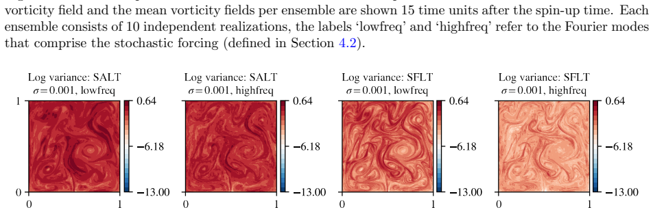
- [§4.1–4.5, Figures 3, 5, 8, 13] The numerical evidence rests on ensembles of only 10 members, with no ensemble-size convergence study and no error bars on the variance maps. The text states that 10 members 'is found to provide a clear insight into the qualitative and quantitative differences', but the palinstrophy and trajectory plots show one-standard-deviation bands whose own sampling error is substantial at this ensemble size. Since the paper makes quantitative statements (e.g., 'the effect of EA SFLT is substantially smaller', §4.3; 'SALT induces variance localized near vorticity gradients'), the absence of sampling-error quantification weakens the empirical support. Please add a convergence check with increasing ensemble size, or at least report bootstrap/standard errors on the key statistics (palinstrophy peak timing, trajectory spread, variance maxima).
minor comments (7)
- [Throughout] The notation k is used both as a wave vector and as a vector component in Eq. (22) ('k = (k,l)^T'); this is confusing. Use e.g. k = (k_1,k_2).
- [Reference [37]] The author name is misspelled as 'Krajchnan'; it should be 'Kraichnan'.
- [§1, last paragraph] The structure description says 'The numerical tests are described in Section 2'; this should be Section 4.
- [Eq. (14)] Minor wording: 'using the integration by parts identity' should be 'using the integration-by-parts identity'.
- [§4.2] The definition of the low-frequency group ('5 ≤ ||k||') is incomplete; it presumably means 5 ≤ ||k|| < 10 or an explicit finite band. Please clarify.
- [Figures 3, 5, 8, 13] The captions say the common logarithm of the variance is shown, but the colorbar labels (e.g., 13.00, 6.61, 0.22) appear to be variance values, not logarithms. Please make the scale unambiguous.
- [§4.5] There is a typo 'SLFT' in the sentence 'individual SLFT realizations remain more closely aligned'; should be 'SFLT'.
Circularity Check
No circularity: the SALT-vs-SFLT scaling is derived from the equations; the Eq. (33) normalization is a transparent amplitude convention and a caveat, not a circular step.
full rationale
The central quantitative comparison is derived in Eqs. (23)-(24) from the defining SALT/SFLT equations (12) and (15) together with the Laplacian eigenrelation omega_k = -4 pi^2 |k|^2 psi_k. This is a mathematical consequence, not an equivalence between input and output: the noise amplitudes are not adjusted to match the reported variance fields, and no parameter is fitted to the numerical data. The numerical experiments in Section 4 use the explicitly stated normalization (32)-(33); they illustrate the analytically expected localization, and the paper itself marks the variance localization as 'by construction' in Section 4.3. The choice theta_k = sigma 4 pi^2 F_k does set the constant prefactor of the ratio, so the precise '|k|^2' phrasing is convention-dependent; however, the qualitative scale-sensitivity persists for any constant relative amplitude and would only be removed by a k-dependent normalization, which is not what the paper does. This is a modeling caveat, not circular reasoning. Self-citations (Holm [28,29], Drivas-Holm-Leahy [13], Alonso-Orán et al. [1]) introduce the frameworks, but all conservation properties used later are re-derived in Eqs. (14) and (17), and no uniqueness theorem or unverified prior is invoked to force the conclusion.
Assumptions & free parameters
free parameters (4)
- SFLT noise amplitude normalization =
4π²
- noise magnitude σ =
0.001 and 0.005
- forcing wavenumber bands =
low: 5 ≤ |k| < 10; high: 10 ≤ |k| ≤ 20
- mollifier cutoff α =
64
assumptions (5)
- domain assumption Simultaneous preservation of kinetic energy and Casimir functions restricts stochastic perturbations to a reparametrization of time, forcing a choice between SALT and SFLT.
- standard math The SALT equations preserve Lie–Poisson structure and Casimirs, and SFLT preserves energy (Eqs. 14 and 17).
- domain assumption The LA SALT expectation equation (19) and EA SFLT expectation equation (21) are the correct closed mean-field dynamics.
- standard math Fourier modes are eigenfunctions of the Laplacian on the torus, and ω_k = -4π²|k|²ψ_k.
- domain assumption The numerical scheme preserves energy and is L²-stable in the absence of diffusion (§4.1).
Cite this review
Pith. "Pith review of Numerical comparison of energy- versus circulation-preserving stochastic vortex dynamics." pith.science (2026). https://pith.science/paper/SUGU6PWI
@misc{pith2026260624275,
  author       = {Pith},
  title        = {Pith review of: Numerical comparison of energy- versus circulation-preserving stochastic vortex dynamics},
  year         = {2026},
  howpublished = {\url{https://pith.science/paper/SUGU6PWI}},
  note         = {Machine review of arXiv:2606.24275}
}
abstract
We compare two geometric stochastic frameworks for the two-dimensional Euler equations, being the circulation-preserving stochastic advection by Lie transport (SALT) and the energy-preserving stochastic forcing by Lie transport (SFLT) approaches. While preserving both circulation and energy is ideal, their simultaneous conservation restricts perturbations to a stochastic reparametrization of time. Consequently, a fundamental choice must be made between preserving structure or the kinetic energy. Analysis reveals that SALT is significantly more sensitive to high-frequency flow components, with noise effects scaling by $| \bk |^2$ relative to SFLT. This suggests that SALT acts as a localized perturbation sensitive to sharp gradients, while SFLT behaves as a more regularized global forcing. Numerical experiments on a traveling dipole, vortex merger, and forced-damped turbulence confirm that SALT introduces uncertainty localized near dynamically active vorticity gradients, whereas SFLT produces a more diffuse variance field spread across the domain. These results illustrate how the choice of geometric invariant fundamentally determines scale-sensitivity and spatial distribution of modeled uncertainty in vortex dynamics.
Figures


Figures from the paper (10 more)




Reference graph
Works this paper leans on
-
[1]
Alonso-Or´ an, A
D. Alonso-Or´ an, A. Bethencourt de Le´ on, D. D. Holm, and S. Takao. Modelling the climate and weather of a 2d lagrangian-averaged euler–boussinesq equation with transport noise.Journal of Statistical Physics, 179(5):1267–1303, 2020
2020
-
[2]
V. Arnold. Sur la g´ eom´ etrie diff´ erentielle des groupes de lie de dimension infinie et ses applications ` a l’hydrodynamique des fluides parfaits. InAnnales de l’institut Fourier, volume 16, pages 319–361, 1966
1966
-
[3]
V. I. Arnold and B. A. Khesin.Topological methods in hydrodynamics. Springer, 1998
1998
-
[4]
Balay, S
S. Balay, S. Abhyankar, M. F. Adams, S. Benson, J. Brown, P. Brune, K. Buschelman, E. Constantinescu, L. Dalcin, A. Dener, V. Eijkhout, J. Faibussowitsch, W. D. Gropp, V. Hapla, T. Isaac, P. Jolivet, D. Karpeev, D. Kaushik, M. G. Knepley, F. Kong, S. Kruger, D. A. May, L. C. McInnes, R. T. Mills, L. Mitchell, T. Munson, J. E. Roman, K. Rupp, P. Sanan, J. ...
2025
-
[5]
Bernsen, O
E. Bernsen, O. Bokhove, and J. J. van der Vegt. A (dis) continuous finite element model for generalized 2D vorticity dynamics.Journal of computational physics, 211(2):719–747, 2006
2006
-
[6]
Chertkov, C
M. Chertkov, C. Connaughton, I. Kolokolov, and V. Lebedev. Dynamics of energy condensation in two-dimensional turbulence.Physical review letters, 99(8):084501, 2007
2007
-
[7]
Cifani, S
P. Cifani, S. Ephrati, and M. Viviani. Sparse-stochastic model reduction for 2D Euler equations. In Stochastic Transport in Upper Ocean Dynamics Annual Workshop, pages 17–28. Springer, 2022
2022
-
[8]
Cifani and F
P. Cifani and F. Flandoli. Diffusion properties of small-scale fractional transport models.Journal of Statistical Physics, 192(11):152, 2025
2025
Show all 46 references
-
[9]
Cifani, F
P. Cifani, F. Flandoli, and L. Marino. Anomalous diffusion properties of stochastic transport by heavy- tailed jump processes.arXiv preprint arXiv:2602.21097, 2026
2026
-
[10]
Cotter, D
C. Cotter, D. Crisan, D. D. Holm, W. Pan, and I. Shevchenko. Modelling uncertainty using stochastic transport noise in a 2-layer quasi-geostrophic model.arXiv preprint arXiv:1802.05711, 2018
2018 arXiv
-
[11]
Cotter, D
C. Cotter, D. Crisan, D. D. Holm, W. Pan, and I. Shevchenko. Numerically modeling stochastic Lie transport in fluid dynamics.Multiscale Modeling & Simulation, 17(1):192–232, 2019
2019
-
[12]
Douglas and T
J. Douglas and T. Dupont. Interior penalty procedures for elliptic and parabolic galerkin methods. In Computing Methods in Applied Sciences: Second International Symposium December 15–19, 1975, pages 207–216. Springer, 2008
1975
-
[13]
T. D. Drivas, D. D. Holm, and J.-M. Leahy. Lagrangian averaged stochastic advection by lie transport for fluids.Journal of Statistical Physics, 179, 2020
2020
-
[14]
M. ´Emery. On two transfer principles in stochastic differential geometry. InS´ eminaire de Probabilit´ es XXIV 1988/89, pages 407–441. Springer, 2006
1988
-
[15]
Ephrati, E
S. Ephrati, E. Jansson, and K. Modin. On spectral scaling laws for averaged turbulence on the sphere. Physica D: Nonlinear Phenomena, 481:134808, 2025
2025
-
[16]
Ephrati, E
S. Ephrati, E. Jansson, and A. Papini. Diffusive behavior of transport noise onS 2.Journal of Compu- tational Dynamics, 14(0):1–16, 2026
2026
-
[17]
S. R. Ephrati. Probabilistic data-driven turbulence closure modeling by assimilating statistics.Journal of Computational Physics, page 114234, 2025
2025
-
[18]
S. R. Ephrati, P. Cifani, E. Luesink, and B. J. Geurts. Data-driven stochastic Lie transport modelling of the 2D Euler equations.Journal of Advances in Modeling Earth Systems, page e2022MS003268, 2023
2023
-
[19]
Flandoli, L
F. Flandoli, L. Galeati, and D. Luo. Scaling limit of stochastic 2d euler equations with transport noises to the deterministic navier–stokes equations.Journal of Evolution Equations, 21(1):567–600, 2021. 25
2021
-
[20]
Flandoli, S
F. Flandoli, S. Morlacchi, and A. Papini. Effect of transport noise on kelvin–helmholtz instability. In Stochastic Transport in Upper Ocean Dynamics Annual Workshop, pages 29–52. Springer, 2022
2022
-
[21]
Freitas, L
A. Freitas, L. Biferale, M. Desbrun, G. Eyink, A. A. Mailybaev, and K. Um. On the importance of stochasticity in closures of turbulence.arXiv preprint arXiv:2602.19875, 2026
2026
-
[22]
L. Galeati. On the convergence of stochastic transport equations to a deterministic parabolic one. Stochastics and Partial Differential Equations: Analysis and Computations, 8(4):833–868, 2020
2020
-
[23]
Gottlieb
S. Gottlieb. On high order strong stability preserving Runge-Kutta and multi step time discretizations. Journal of scientific computing, 25(1):105–128, 2005
2005
-
[24]
D. A. Ham, P. H. J. Kelly, L. Mitchell, C. J. Cotter, R. C. Kirby, K. Sagiyama, N. Bouziani, S. Vorder- wuelbecke, T. J. Gregory, J. Betteridge, D. R. Shapero, R. W. Nixon-Hill, C. J. Ward, P. E. Farrell, P. D. Brubeck, I. Marsden, T. H. Gibson, M. Homolya, T. Sun, A. T. T. Mc...
2023
-
[25]
Hasselmann
K. Hasselmann. Stochastic climate models part i. theory.tellus, 28(6):473–485, 1976
1976
-
[26]
D. Holm, R. Hu, and O. Street. Deterministic and stochastic geometric mechanics for hall magneto- hydrodynamics.Proceedings of the Royal Society A: Mathematical, Physical and Engineering Sciences, 480(2300), 2024
2024
-
[27]
Holm and J
D. Holm and J. Woodfield. Comparing two different types of stochastic parametrization in geophysical flow.Physics of Fluids, 36(11), 2024
2024
-
[28]
D. D. Holm. Variational principles for stochastic fluid dynamics.Proceedings of the Royal Society A: Mathematical, Physical and Engineering Sciences, 471(2176):20140963, 2015
2015
-
[29]
D. D. Holm, E. Luesink, and W. Pan. Stochastic mesoscale circulation dynamics in the thermal ocean. Physics of Fluids, 33(4):046603, 04 2021
2021
-
[30]
D. D. Holm, J. E. Marsden, and T. S. Ratiu. Euler–Poincar´ e models of ideal fluids with nonlinear dispersion.Physical Review Letters, 80(19):4173, 1998
1998
-
[31]
D. D. Holm and W. Pan. Deterministic and stochastic euler–boussinesq convection.Physica D: Nonlinear Phenomena, 444:133584, 2023
2023
-
[32]
D. D. Holm, M. K. Singh, and O. D. Street. A comparative numerical study of stochastic Hamiltonian Camassa–Holm equations.Proceedings of the Royal Society A: Mathematical, Physical and Engineering Sciences, 482(2330), 2026
2026
-
[33]
Houston, C
P. Houston, C. Schwab, and E. S¨ uli. Discontinuous hp-finite element methods for advection-diffusion- reaction problems.SIAM Journal on Numerical Analysis, 39(6):2133–2163, 2002
2002
-
[34]
Hu and S
R. Hu and S. Patching. Variational stochastic parameterisations and their applications to primitive equation models. InStochastic Transport in Upper Ocean Dynamics Annual Workshop, pages 135–158. Springer, 2021
2021
-
[35]
P. E. Kloeden and R. Pearson. The numerical solution of stochastic differential equations.The ANZIAM Journal, 20(1):8–12, 1977
1977
-
[36]
R. H. Kraichnan. Anomalous scaling of a randomly advected passive scalar.Physical review letters, 72(7):1016, 1994
1994
-
[37]
F. H. Krajchnan. Inertial ranges in two-dimensional turbulence.The Physics of Fluids, 10:1417, 1967
1967
-
[38]
Lahaye, O
N. Lahaye, O. Larroque, and V. Zeitlin. Equatorial modons in thermal rotating shallow water model. Journal of Fluid Mechanics, 984:A58, 2024
2024
-
[39]
Lahaye and V
N. Lahaye and V. Zeitlin. Coherent magnetic modon solutions in quasi-geostrophic shallow water mag- netohydrodynamics.Journal of Fluid Mechanics, 941:A15, 2022. 26
2022
-
[40]
J. E. Marsden, T. S. Ratiu, and M. Golubitsky.Introduction to mechanics and symmetry: a basic exposition of classical mechanical systems, volume 17. Springer, 1999
1999
-
[41]
Modin and M
K. Modin and M. Viviani. A brief introduction to matrix hydrodynamics.arXiv preprint arXiv:2508.07088, 2025
2025
-
[42]
P. Saffman. The approach of a vortex pair to a plane surface in inviscid fluid.Journal of Fluid Mechanics, 92(3):497–503, 1979
1979
-
[43]
K. K. Sharma and P. Korn. Structure-preserving stochastic parameterization of a barotropic coupled ocean-atmosphere model with ornstein–uhlenbeck noise.arXiv preprint arXiv:2603.26693, 2026
2026
-
[44]
Woodfield
J. Woodfield. Strong stability preservation for stochastic partial differential equations.arXiv preprint arXiv:2411.11172, 2024
2024 arXiv
-
[45]
Zeitlin.Geophysical fluid dynamics: understanding (almost) everything with rotating shallow water models
V. Zeitlin.Geophysical fluid dynamics: understanding (almost) everything with rotating shallow water models. Oxford University Press, 2018
2018
-
[46]
Zhong and J
G. Zhong and J. E. Marsden. Lie-poisson hamilton-jacobi theory and lie-poisson integrators.Physics Letters A, 133(3):134–139, 1988. 27
1988
Reviewed August 2, 2026 · model on record in the stance chip above.
Discussion (0). Continue with ORCID to comment.