Critical Decisions for Asset Allocation via Penalized Quantile Regression

Giovanni Bonaccolto

REVIEW 2 major objections 5 minor 37 references

Critical Decisions for Asset Allocation via Penalized Quantile Regression

T0 review · 2 major / 5 minor · reviewed 2026-08-14 · deepseek-v4-flash

Challenge this review Re-run · record.json Download PDF Read on arXiv ↗ Review JSON

Pith's one-line read Adding a post-LASSO re-estimation step to penalized quantile regression yields portfolios with lower expected shortfall and volatility than simple LASSO or equal weights.

desk verdict A useful empirical extension of penalized quantile regression portfolios, but the headline ES claim rests on point estimates without inference and needs a revision before the paper's central conclusion can be trusted. read the letter →

arxiv 1908.04697 v1 pith:SYCT7756 submitted 2019-08-13 q-fin.PM

Giovanni Bonaccolto This is my paper · ORCID

classification q-fin.PM

keywords PenalizedquantileregressionPost-LASSOExpectedshortfallPortfoliooptimizationAssetallocationTuningparameterselectionSCADMCP

verification ladder T0 review T1 audit T2 compute T3 formal

The pith

A machine-rendered reading of the paper's core claim, the machinery that carries it, and where it could break.

The reading

The paper asks whether the standard LASSO version of quantile-regression portfolio selection leaves performance on the table, and it argues that a two-step post-LASSO version does. In the first step, a penalized quantile regression selects a small set of assets; in the second, the selected assets are re-weighted by an unpenalized quantile regression. Across weekly returns on 49 industry portfolios and 100 size/book-to-market portfolios, the post-LASSO strategy with the Belloni-Chernozhukov tuning rule records the lowest out-of-sample expected shortfall in almost every configuration, lower volatility, and higher accumulated wealth than the equally weighted benchmark. A sympathetic reader would care because the equally weighted portfolio is notoriously hard to beat, and the improvement comes with no extra estimation burden. The paper also finds that nonconvex penalties (SCAD, MCP) beat plain LASSO in several cases, but the post-LASSO step is the main driver.

What carries the argument

The load-bearing object is the penalized quantile regression objective $\arg\min_{(w,\mu)} \frac{1}{T}\sum_t \rho_\tau(x_{s,t}-\sum_j w_j x_{j,t}-\mu) + \frac{\lambda\sqrt{\tau(1-\tau)}}{T}\sum_j \hat\sigma_j |w_j|$, where $\rho_\tau(u)=u(\tau-\mathbf{1}_{u<0})$ is the quantile check loss and the $x_{j,t}$ are spreads between the reference asset's return and each other asset's return, so the coefficients are portfolio weights. The post-LASSO machinery then takes the coefficients from that problem, keeps only assets with $|w_j|>\eta$, and re-estimates their weights from the unpenalized check-loss problem; discarded weights are set to zero. That second step is what removes the overshrinking of the selected coefficients and the resulting overweighting of the reference asset. The Belloni-Chernozhukov rule supplies the tuning parameter by a data-driven computation, and is compared against a BIC designed for quantile regression and 5-fold cross-validation.

What would settle it

Keep PLBCH's method identical but replace the reference-picking rule with a fixed stock or with the lowest-volatility stock; if PLBCH stops beating equal weighting on expected shortfall and wealth in most configurations, the finding is tied to the reference choice rather than to the post-LASSO mechanism.

Watch

Extended reading notes

Core claim

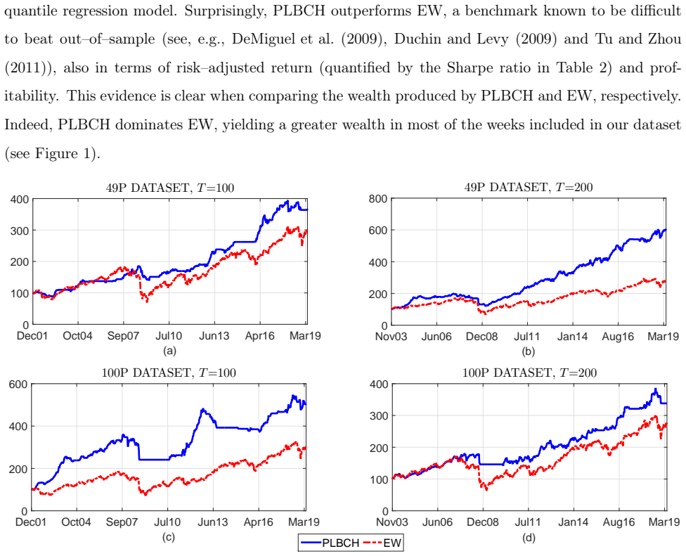
The central claim is that the post-LASSO quantile regression rule labeled PLBCH—first solve the $\ell^1$-penalized quantile regression with the data-driven tuning parameter, discard coefficients below a threshold, then re-estimate the surviving weights without penalty—outperforms the simple LASSO quantile-regression strategy and the equally weighted portfolio out of sample. The evidence is strongest on the risk dimension: PLBCH produces the lowest expected shortfall at the 5% level in three of four dataset/window configurations, the lowest standard deviation in three of four, and higher wealth than equal weighting in most weeks. The paper also claims the post-LASSO step fixes a concentration problem: the weight on the asset chosen as the response variable falls from an average of 0.9310 to 0.3621 in one configuration. Comparisons of convex versus nonconvex penalties and of three tuning-parameter rules are secondary; the post-penalization re-estimation is the decisive change.

Load-bearing premise

The model always picks, in each training window, the single stock with the lowest expected shortfall inside that window as the reference around which the portfolio is built; if that pick is unstable or overfitted, the reported gains could vanish.

Editorial extensions

If this is right

If PLBCH's out-of-sample ranking holds, investors who optimize portfolios by tail risk can lower expected shortfall and volatility without sacrificing return: PLBCH beats the equally weighted benchmark on Sharpe ratio in the 49P configurations and generates more wealth over most of the sample.
The post-LASSO step is cheap: the paper reports mean runtimes per rolling window under a tenth of a second for LBCH and only modest increases for PLBCH, so the improvement is available at negligible computational cost.
The concentration problem identified in the earlier LASSO version is mitigated: the reference asset's average weight drops from 0.9310 to 0.3621, which makes the portfolios more balanced and easier to hold.
Penalty choice matters less than the two-step re-estimation when the goal is tail risk; SCAD and MCP provide some gains over LASSO under cross-validation, but post-penalization is the consistent driver of lower expected shortfall.
The tuning rule and the estimation step interact rather than acting independently: without post-LASSO, cross-validation can beat the Belloni-Chernozhukov rule, while with post-LASSO the Belloni-Chernozhukov rule is usually best.

Reading between the lines

Editorial extensions of the paper, not claims the author makes directly.

A testable extension the paper does not run: replace the lowest-in-sample-ES choice of reference asset with a fixed asset or a rule based on liquidity; if the PLBCH edge over equal weighting shrinks, the reported gains are partly an artifact of that selection rule rather than of post-LASSO itself.
Because the post-LASSO step reduces the reference asset's weight, it behaves like an implicit exposure cap; combining it with explicit gross-exposure constraints could yield even lower concentration at the cost of some tail-risk reduction.
The results are estimated at the 5% quantile only; the paper itself suggests other quantile levels. One would expect the ES advantage to be largest exactly at the quantile being optimized, so a natural check is whether PLBCH still dominates at 1% or 10% tails.
The same two-step recipe transfers outside portfolios: any penalized quantile regression used for variable selection, such as factor-based risk models, could benefit from re-estimating selected coefficients without shrinkage.

Share X Bluesky LinkedIn Reddit HN

Signed reviews

No signed human review yet.

Editorial analysis

A structured set of objections, weighed in public.

Desk editor's note, referee report, and a circularity audit.

Desk Editor's Note

read the letter

Short version: this is a solid empirical extension, not a breakthrough. The paper's real contribution is the first combination of post-LASSO re-estimation, nonconvex penalties (SCAD, MCP), and alternative tuning rules (BCH, BIC, CV5) in quantile-regression-based portfolio construction. That combination is new, the empirical setup is standard and clearly described, and the two datasets with rolling windows give the comparison a reasonable basis. The post-LASSO step does what it claims: it reduces portfolio concentration and the weight on the reference asset, and the reported out-of-sample ES and volatility improvements over plain LASSO are directionally credible. The runtime numbers are also a nice practical touch.

The soft spots are real but mostly concentrated in one place. The paper's strongest claim—that PLBCH generates the lowest ES in all but one case—is never tested for significance. The Ledoit-Wolf tests cover variance and Sharpe ratio only, and the Sharpe differences are mostly insignificant anyway. The ES estimator is based on roughly 40–45 tail observations per panel, so the gaps in Table 2 (sometimes under 0.2 percentage points) could easily be sampling noise. The text in Section 4 says ES values 'significantly decrease' after post-penalization, but no test supports that. That is a load-bearing issue for the headline, not a cosmetic one.

Your reader's other concern also lands: the response asset is chosen as the one with the lowest in-sample ES in each rolling window. That makes the reference asset data-dependent and potentially unstable; it also means the reported gains are conditional on that particular selection rule. It is not fatal, but it should be disclosed more prominently and ideally checked under alternative selection rules.

One thing I disagree with in the reader's take: the circularity burden is low. This is an empirical horse race against external benchmarks, not a derivation that reduces to a fitted quantity. Self-citation of the author's prior LASSO-quantile-regression work is legitimate here because that is the baseline being extended. The lack of released code and data is a minor issue given the datasets are public, but a fixed-seed replication script would make the comparison much more convincing.

Bottom line: this paper deserves a serious referee. It is a competent empirical contribution to a niche but active literature, and the post-LASSO insight is worth testing further. The revision needs significance tests for ES differences (bootstrap or Ledoit-Wolf-style), a multiple-testing disclosure, and ideally code plus seed. With those, I would cite it.

Referee Report

2 major / 5 minor

Summary. The manuscript studies portfolio construction via penalized quantile regression. It proposes a post-penalization two-step procedure in which LASSO, SCAD, or MCP penalties are used for variable selection, after which a nonpenalized quantile regression is fitted on the selected assets, and it compares tuning-parameter selection by the Belloni-Chernozhukov method, a BIC, and 5-fold cross-validation. Using weekly returns for the 49 Industry Portfolios and the 100 size/book-to-market portfolios, with rolling windows of T = 100 and T = 200 and τ = 0.05, the paper reports out-of-sample expected shortfall, standard deviation, Sharpe ratio, turnover, and active/short positions. The headline result is that PLBCH (post-LASSO with Belloni-Chernozhukov tuning) delivers the lowest expected shortfall in all but one of the four configurations, together with lower volatility and lower portfolio concentration than simple LASSO and than the equally weighted benchmark.

Significance. If the empirical claims are adequately supported, the paper offers a practically useful extension of penalized quantile regression for asset allocation by showing that a two-step post-LASSO estimator can mitigate the response-asset overweighting documented in Bonaccolto et al. (2018) and improve tail-risk performance, while remaining computationally cheap. The comparison against the equally weighted portfolio is a meaningful stress test, and the reporting of turnover and active/short positions helps assess implementability. The experimental grid of two datasets and two window lengths is reasonable, and the computational runtime comparisons are useful. However, the central risk comparison currently lacks inferential support, and the data-dependent construction of the response asset deserves explicit robustness analysis.

major comments (2)

[Section 4, Table 2] The claim that PLBCH generates the lowest ES, and the statement that 'the values of ES significantly decrease' when moving to post-penalized strategies, are supported only by point estimates. Tables 3 and 4 report Ledoit and Wolf (2008) tests for variances and Sharpe ratios, but not for ES, which is the paper's target measure. With Q − T ∈ {806, 906} out-of-sample weeks and τ = 0.05, the ES in Eq. (11) is estimated from roughly 40–45 tail observations, so sampling variability is non-negligible; for example, in Panel (d) the PLBCH advantage over the second-best strategy is about 0.15 percentage points. The authors should provide standard errors, bootstrap confidence intervals, or a formal test for ES differences, ideally with a multiple-testing correction, before claiming that PLBCH is 'lowest' or that ES 'significantly decreases.'
[Section 3, response-asset selection] The response variable xs,t is defined as the return of the asset with the lowest in-sample expected shortfall in each rolling window. Because this is the same risk measure that the quantile-regression objective targets, the reported ES figures are conditional on a data-dependent order statistic whose identity can change across windows. The paper gives no information on how often the reference asset changes, nor any robustness analysis with a fixed reference asset or an alternative selection rule. Without such diagnostics, it is unclear whether the ES advantage of PLBCH is a property of the post-LASSO estimator or an artifact of the specific reference-asset selection. Please report the frequency of reference-asset changes over the rolling windows and add at least one alternative selection rule as a robustness check.

minor comments (5)

[Throughout] Typographical issues such as 'state–of–art' and the title spacing in 'Quan tile Regression' should be corrected.
[Table 2] The Sharpe ratios are reported with a percent sign, but the units are not otherwise defined; please clarify the scaling in the table notes.
[Figure 1] The axis tick labels are compressed and difficult to read, and the subfigure labels in the caption should be explicitly matched to panels (a)–(d).
[Section 4] The paper reports turnover but does not compute net-of-transaction-cost performance; a brief statement about whether the qualitative conclusions survive plausible transaction costs would strengthen the practical claims.
[Data and code] No data or code availability statement is provided; making the R scripts available would substantially aid reproducibility.

Circularity Check

0 steps flagged · score 0.0 of 10

No significant circularity: the reported ES ranking is an out-of-sample empirical result, not a construction from the fitted inputs.

full rationale

The paper's central claims are empirical out-of-sample comparisons of portfolio rules (ES, SD, SR) against each other and against the equally weighted benchmark. PLBCH is constructed by a first-step LASSO selection with Belloni-Chernozhukov tuning and a second-step unpenalized quantile regression in Eq. (5); the reported ES in Eq. (11) is computed from held-out returns rp,t+1, not from the in-sample objective. The only potentially self-referential design element is the choice of the response asset as the one with the lowest in-sample expected shortfall, taken from Bonaccolto et al. (2018); this is a shared input for all regression-based strategies, including the simple LASSO benchmark, so it cannot by construction make PLBCH's ES lower than LBCH's. No uniqueness theorem is imported from the authors' prior work, and no ansatz is smuggled via citation: post-LASSO, BCH, BIC, CV5, SCAD, and MCP are all implemented as standard methods with external citations. The absence of significance tests for ES is a robustness and correctness limitation, not a circularity.

Assumptions & free parameters 5 free parameters · 6 assumptions · 0 invented entities

This ledger captures every input the central claim depends on that is not derived in the paper. The key free choices are the tuning parameters (lambda, eta, tau, and the constants B, c, 1-beta, CT, K), all of which are user-set. The mathematical background (QR to ES minimization, budget-constrained return decomposition, validity of the BCH and BIC rules) is imported from the cited literature. No new theoretical entities are posited, so invented_entities is empty.

free parameters (5)

lambda (penalty intensity) = Selected per rolling window via BCH, BIC, or CV5; grid of 100 values
Controls sparsity of the portfolio weights in eq (2). The paper compares three selection rules and reports that the choice strongly affects performance (Section 2, Table 2).
eta (post-penalization selection threshold) = 1e-5
Regressors with |w_j| <= eta are discarded in the first step; it also defines active and short positions in eqs (14)-(15) (Section 3).
tau (quantile / ES level) = 0.05
Sets the risk target and the regression loss; a manual modeling choice (Section 3).
B, c, 1-beta (BCH tuning constants) = B=1000, c=2, 1-beta=0.9
Set on the recommendation of Belloni and Chernozhukov (2011); c scales the penalty in eq (4).
CT (BIC constant) and K (CV folds) = CT = log T; K = 5
Set following Lee et al. (2014) and Hastie et al. (2009); both influence the selected lambda and the reported performance.

assumptions (6)

standard math Minimizing the quantile regression check loss at level tau yields the portfolio with minimum expected shortfall at level tau (Bassett et al., 2004).
Background result linking QR to ES minimization, used to justify the objective in eq (2).
standard math The portfolio return can be rewritten as rp,t = xs,t - sum_{j != s} wj xj,t under the budget constraint ws = 1 - sum wj (Fan et al., 2012).
Reduces the constrained portfolio problem to an unconstrained regression, eq (1).
domain assumption The Belloni-Chernozhukov data-driven lambda, lambda* = c * Lambda(1-beta|X), provides a valid penalty level for high-dimensional sparse quantile regression.
Theoretical property from Belloni and Chernozhukov (2011); the paper imports it as a black box and relies on it for PLBCH.
domain assumption The Lee et al. (2014) BIC with asymmetric Laplace errors is consistent for quantile regression model selection.
Imported from Lee et al. (2014) and used to choose lambda in PLBIC.
domain assumption K-fold cross-validation on the check loss selects lambda for out-of-sample performance.
Standard heuristic (Hastie et al., 2009); the paper uses it for LCV5, SCV5, MCV5 and post-penalized variants.
domain assumption Rolling-window out-of-sample evaluation on the 2000-2019 sample is representative of real-time portfolio performance.
The empirical conclusions are drawn from a single historical sample with no guarantee of stationarity or representativeness.

how reviews work

0 comments

Cite this review

Pith. "Pith review of Critical Decisions for Asset Allocation via Penalized Quantile Regression." pith.science (2026). https://pith.science/paper/SYCT7756

@misc{pith2026190804697,
  author       = {Pith},
  title        = {Pith review of: Critical Decisions for Asset Allocation via Penalized Quantile Regression},
  year         = {2026},
  howpublished = {\url{https://pith.science/paper/SYCT7756}},
  note         = {Machine review of arXiv:1908.04697}
}

read the original abstract

We extend the analysis of investment strategies derived from penalized quantile regression models, introducing alternative approaches to improve state\textendash of\textendash art asset allocation rules. First, we use a post\textendash penalization procedure to deal with overshrinking and concentration issues. Second, we investigate whether and to what extent the performance changes when moving from convex to nonconvex penalty functions. Third, we compare different methods to select the optimal tuning parameter which controls the intensity of the penalization. Empirical analyses on real\textendash world data show that these alternative methods outperform the simple LASSO. This evidence becomes stronger when focusing on the extreme risk, which is strictly linked to the quantile regression method.

Figures

Figures reproduced from arXiv: 1908.04697 by the authors.

Discussion (0). Continue with ORCID to comment.

Reference graph

Works this paper leans on

37 extracted references · 32 canonical work pages

[1]

Acerbi, C. and D. Tasche (2002). Expected shortfall: A natural coherent alternative to value at risk. Economic Notes\/ 31\/ (2), 379--388

work page 2002
[2]

Delbaen, J

Artzner, P., F. Delbaen, J. Eber, and D. Heath (1999). Coherent measures of risk. Mathematical Finance\/ 9\/ (3), 203--228

work page 1999
[3]

Assa, H. (2015). Risk management under a prudential policy. Decisions in Economics and Finance\/ 38\/ (2), 217–230

work page 2015
[4]

Koenker, and G

Bassett, G., R. Koenker, and G. Kordas (2004). Pessimistic portfolio allocation and choquet expected utility. Journal of Financial Econometrics\/ 2\/ (4), 477--492

work page 2004
[5]

Belloni, A. and V. Chernozhukov (2011). L1-penalized quantile regression in high-dimensional sparse models. The Annals of Statistics\/ 39\/ (1), 82--130

work page 2011
[6]

Caporin, and S

Bonaccolto, G., M. Caporin, and S. Paterlini (2018). Asset allocation strategies based on penalized quantile regression. Computational Management Science\/ 15\/ (1), 1--32

work page 2018
[7]

Bonaccolto, G. and S. Paterlini (2019). Developing new portfolio strategies by aggregation. Annals of Operations Research\/ (forthcoming)

work page 2019
[8]

Daubechies, C

Brodie, J., I. Daubechies, C. D. Mol, D. Giannone, and I. Loris (2009). Sparse and stable markowitz portfolios. PNAS\/ 106\/ (30), 12267--12272

work page 2009

Show all 37 references

[9]

Chen, S. X. (2008). Nonparametric estimation of expected shortfall. Journal of Financial Econometrics\/ 6\/ (1), 87--107

2008
[10]

Kondor, and M

Ciliberti, S., I. Kondor, and M. Mézard (2007). On the feasibility of portfolio optimization under expected shortfall. Quantitative Finance\/ 7\/ (4), 389--396

2007
[11]

Garlappi, F

DeMiguel, V., L. Garlappi, F. J. Nogales, and R. Uppal (2009). A generalized approach to portfolio optimization: Improving performance by constraining portfolio norms. Management Science\/ 55\/ (5), 798--812

2009
[12]

Garlappi, and R

DeMiguel, V., L. Garlappi, and R. Uppal (2009). Optimal versus naive diversification: How inefficient is the 1/N portfolio strategy? Review of Financial Studies\/ 22 , 1915--1953

2009
[13]

Duchin, R. and H. Levy (2009). Markowitz versus the talmudic portfolio diversification strategies. Journal of Portfolio Management\/ 35 , 71--74

2009
[14]

Fan, J. and R. Li (2001). Variable selection via nonconcave penalized likelihood and its oracle properties. Journal of the American Statistical Association\/ 96\/ (456), 1348--1360

2001
[15]

Zhang, and K

Fan, J., J. Zhang, and K. Yu (2012). Vast portfolio selection with gross-exposure constraints. Journal of the American Statistical Association\/ 107\/ (498), 592--606

2012
[16]

Paterlini, and P

Fastrich, B., S. Paterlini, and P. Winker (2015). Constructing optimal sparse portfolios using regularization methods. Computational Management Science\/ 12\/ (3), 417--434

2015
[17]

Gijbels, I. and K. Herrmann (2018). Optimal expected-shortfall portfolio selection with copula-induced dependence. Applied Mathematical Finance\/ 25\/ (1), 66--106

2018
[18]

Gilli, M. and E. Këllezi (2002). A global optimization heuristic for portfolio choice with VaR and E xpected S hortfall. In E. J. Kontoghiorghes, B. Rustem, and S. Siokos (Eds.), Computational Methods in Decision-Making, Economics and Finance. Applied Optimization , Volume 74,...

2002
[19]

Giuzio, M. (2017). Genetic algorithm versus classical methods in sparse index tracking. Decisions in Economics and Finance\/ 40\/ (1-2), 243–256

2017
[20]

Giuzio, M. and S. Paterlini (2018). Un diversifying during crises: is it a good idea? Computational Management Science\/ 16\/ (3), 401--432

2018
[21]

Tibshirani, and J

Hastie, T., R. Tibshirani, and J. Friedman (2009). The Elements of Statistical Learning . Springer

2009
[22]

Schaumburg, and M

Hautsch, N., J. Schaumburg, and M. Schienle (2014). Financial network systemic risk contributions. Review of Finance\/ 19\/ (2), 685–738

2014
[23]

Koenker, R. (2005). Quantile regression . Number 38. Cambridge university press

2005
[24]

Koenker, R. and G. Bassett (1978). Regression quantiles. Econometrica\/ 46\/ (1), 33--50

1978
[25]

Kratz, M., Y. H. Lok, and A. J. McNeil (2018). Multinomial VaR backtests: a simple implicit approach to backtesting expected shortfall. Journal of Banking & Finance\/ 88 , 393--407

2018
[26]

Kremer, P. J., A. Talmaciu, and S. Paterlini (2018). Risk minimization in multi factor portfolios: what is the best strategy? Annals of Operations Research\/ 266\/ (1-2), 255--291

2018
[27]

Ledoit, O. and M. Wolf (2008). Robust performance hypothesis testing with the S harpe ratio. Journal of Empirical Finance\/ 15\/ (5), 850--859

2008
[28]

Lee, E. R., H. Noh, and B. U. Park (2014). Model selection via B ayesian information criterion for quantile regression models. Journal of the American Statistical Association\/ 109\/ (505), 216--229

2014
[29]

Li, Y. and J. Zhu (2008). L1-norm quantile regression. Journal of Computational and Graphical Statistics\/ 17\/ (1), 163--185

2008
[30]

Markowitz, H. (1952). Portfolio selection. The Journal of Finance\/ 7 , 77--91

1952
[31]

Patton, A. J., J. F. Ziegel, and R. Chen (2019). Dynamic semiparametric models for expected shortfall (and V alue at R isk). Journal of Econometrics\/ 211\/ (2), 388 -- 413

2019
[32]

Rockafellar, R. and S. Uryasev (2000). Optimization of conditional var. Journal of Risk\/ 2\/ (3), 21--41

2000
[33]

Tibshirani, R. (1996). Regression analysis and selection via the lasso. Journal of the Royal Statistical Society, Series B\/ 58\/ (1), 267--288

1996
[34]

Tu, J. and G. Zhou (2011). Markowitz meets T almud: A combination of sophisticated and naive diversification strategies. Journal of Financial Economics\/ 99\/ (1), 204--215

2011
[35]

Yamai, Y. and T. Yoshiba (2005). Value at risk versus expected shortfall: a practical perspective. Journal of Banking & Finance\/ 29\/ (4), 997--1015

2005
[36]

Yen, Y. and T. Yen (2014). Solving norm constrained portfolio optimization via coordinate-wise descent algorithms. Computational Statistics and Data Analysis\/ 76 , 737--759

2014
[37]

Zhang, C.-H. (2010). Nearly unbiased variable selection under minimax concave penalty. The Annals of Statistics\/ 38\/ (2), 894--942

2010

Pith tools

Reviewed August 14, 2026 · model on record in the stance chip above.

[1] [1]

Acerbi, C. and D. Tasche (2002). Expected shortfall: A natural coherent alternative to value at risk. Economic Notes\/ 31\/ (2), 379--388

work page 2002

[2] [2]

Delbaen, J

Artzner, P., F. Delbaen, J. Eber, and D. Heath (1999). Coherent measures of risk. Mathematical Finance\/ 9\/ (3), 203--228

work page 1999

[3] [3]

Assa, H. (2015). Risk management under a prudential policy. Decisions in Economics and Finance\/ 38\/ (2), 217–230

work page 2015

[4] [4]

Koenker, and G

Bassett, G., R. Koenker, and G. Kordas (2004). Pessimistic portfolio allocation and choquet expected utility. Journal of Financial Econometrics\/ 2\/ (4), 477--492

work page 2004

[5] [5]

Belloni, A. and V. Chernozhukov (2011). L1-penalized quantile regression in high-dimensional sparse models. The Annals of Statistics\/ 39\/ (1), 82--130

work page 2011

[6] [6]

Caporin, and S

Bonaccolto, G., M. Caporin, and S. Paterlini (2018). Asset allocation strategies based on penalized quantile regression. Computational Management Science\/ 15\/ (1), 1--32

work page 2018

[7] [7]

Bonaccolto, G. and S. Paterlini (2019). Developing new portfolio strategies by aggregation. Annals of Operations Research\/ (forthcoming)

work page 2019

[8] [8]

Daubechies, C

Brodie, J., I. Daubechies, C. D. Mol, D. Giannone, and I. Loris (2009). Sparse and stable markowitz portfolios. PNAS\/ 106\/ (30), 12267--12272

work page 2009