REVIEW 4 major objections 6 minor 36 references
Approximating Spatial Distance Through Confront Networks: Application to the Segmentation of Medieval Avignon
T0 review · 4 major / 6 minor · reviewed 2026-08-12 · deepseek-v4-flash
Pith's one-line read A graph built from medieval 'next-door' mentions reproduces city distances well enough to split Avignon into 31 lived neighborhoods without a single exact address.
desk verdict A useful graph-extraction pipeline for incomplete medieval land records, honestly presented but with a partly self-referential validation—worth refereeing, though the 0.80 correlation should not be read as independent confirmation. read the letter →
The pith
A machine-rendered reading of the paper's core claim, the machinery that carries it, and where it could break.
The reading
What carries the argument
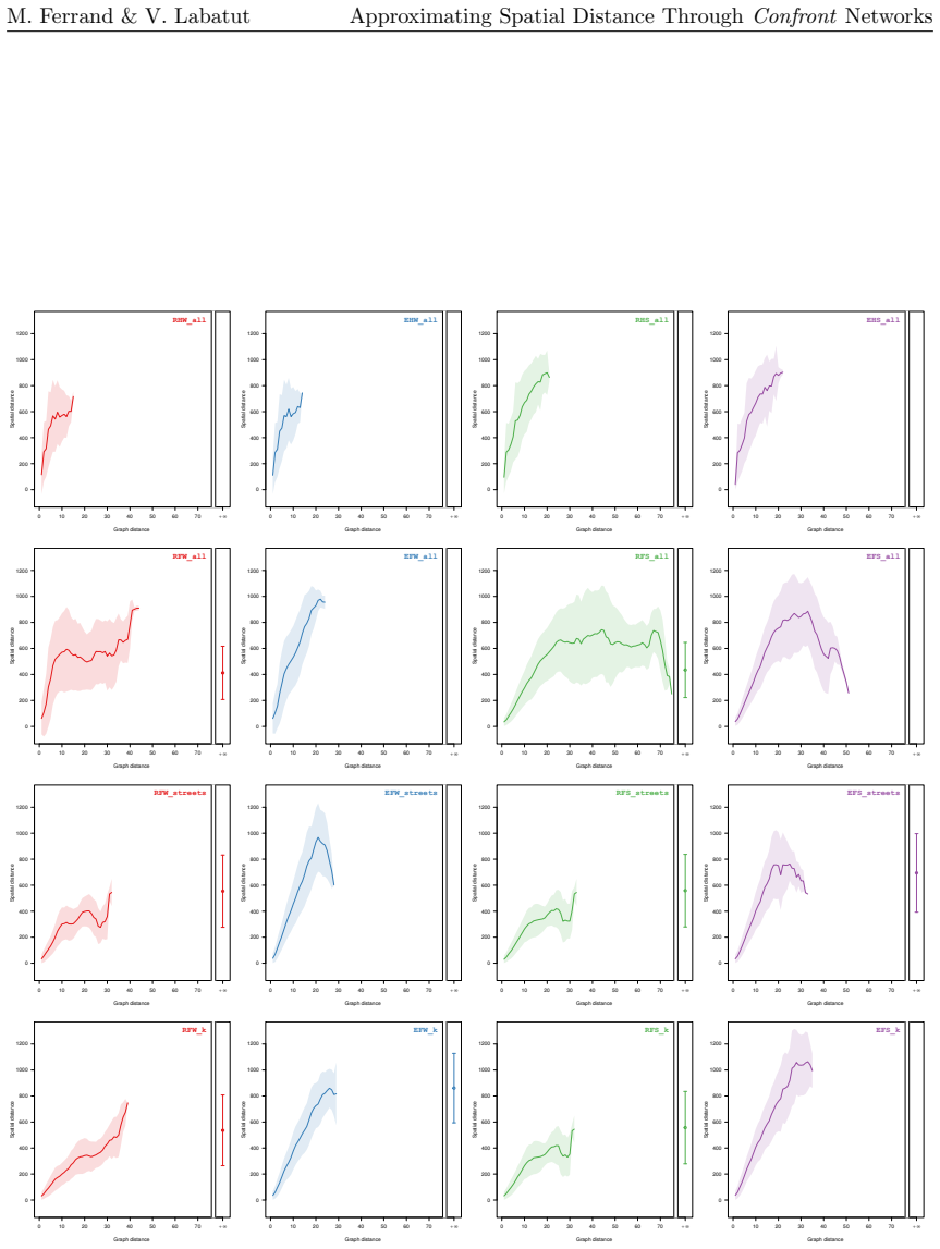
The load-bearing object is the confront network: an undirected spatial graph whose vertices are properties and urban invariants (streets, gates, churches, walls, river) and whose edges are the relative locations recorded in terriers, normalized to seven relation types. The distance-correlation criterion $\rho_d$—Spearman's rank correlation between shortest-path (graph) distance and Euclidean (spatial) distance on the georeferenced subset—carries the method comparison; the paper's extraction variants are essentially attempts to make geodesic distance on the graph behave like Euclidean distance. The best variant, EFS_k, combines extended secondary data, flat relationships only, and splitting of the seven longest streets into artificially connected segments, which prevents long linear objects from acting as spatial shortcuts.
What would settle it
Take the EFS_k extraction, restrict the evaluation to a control set of properties whose medieval positions are independently fixed by surviving archaeology or standing landmarks (churches, gates, walls), and recompute the Spearman correlation; a large drop from 0.80 would show the reported spatial fidelity was an artifact of the confront-based georeferencing loop.
Extended reading notes
Core claim
The paper's central claim is that a confront network—a graph whose edges are the spatial relationships tenants themselves declared (x is north of y, x faces y, x is inside borough z)—is a legitimate stand-in for a map of the urban space, for the purpose of spatial segmentation. The authors define the quality of such a graph by two criteria: coverage (how many of the 3,021 recorded properties the graph retains) and reliability (Spearman rank correlation between graph distance and spatial distance over the 2,049 georeferenced properties). Comparing 16 extraction variants, they find that the best graph is not the one that uses all available information but the one that discards hierarchical containment edges, splits the longest streets, and adds relationships from secondary sources; this EFS_k variant reaches 0.80 correlation while keeping 69% of properties. Partitioning that graph with Louvain produces 31 communities with modularity 0.93, which the authors interpret as the lived neighborhoods of papal Avignon, grounded in spatial proximity and shared landmarks rather than administrative parish lines.
Load-bearing premise
The method's yardstick is not fully independent: the 2,049 property positions used to test distance accuracy were themselves inferred from the same neighbor relationships that build the graph, so part of the 0.80 match may be the method measuring its own input.
Editorial extensions
If this is right
- Historians can segment an incompletely documented city without parcel-by-parcel georeferencing, as long as the registers contain explicit relative locations.
- Discarding hierarchical containment edges and splitting long streets improves distance fidelity; keep-all-information graphs are spatially misleading, with the full graph reaching only 0.22 correlation versus 0.80 for EFS_k.
- Secondary information about how streets connect to each other and to buildings is worth collecting: adding it raised correlation by 0.26 to 0.45 across comparable variants while also improving property coverage.
- The 31 Louvain communities of the best graph form spatially coherent units that cross parish boundaries only at uncertain edges, and typically coalesce around a street, market, cemetery, or borough—consistent with neighborhoods as lived spaces, not administrative cells.
Reading between the lines
- A transferable benchmark design: other cities with terrier-like registers, where cardinal relations may be rare, could reuse the same 'coverage plus distance correlation' selection protocol, but the optimal trade-off will likely shift with the relation types present in the source.
- The 0.80 ceiling is probably not a limit of the method but of the noisy ground truth: the georeferenced properties were manually arranged using the same confronts that make the edges, so part of the measured correlation is circular; an independent control group of properties located via fixed landmarks would reveal the true floor.
- The same graph could feed interpolation of missing absolute positions: instead of averaging neighbor coordinates, a graph neural network could use the edge semantics to predict locations, a perspective the authors mention; if that works, the confront network becomes a scaffold for full georeferencing, not just segmentation.
- The finding that deleting information improves spatial fidelity is likely general: in any spatial graph, hubs representing broad regions collapse many real meters into two hops, so flat plus split representations are a safer default for distance-based analysis on relational sources.
Editorial analysis
A structured set of objections, weighed in public.
Referee Report
Summary. The paper proposes a graph-based approach to representing medieval urban space from land registries, where properties are located only by relative spatial references ('confronts'). Sixteen variants of a confront-network extraction pipeline are compared on a dataset of papal-period Avignon, using two criteria: coverage (number of properties retained in the graph) and reliability (Spearman correlation between graph distance and Euclidean spatial distance). The method EFS_k (extended data, flat relationships, split longest streets) is selected, achieving ρ_d = 0.80, and Louvain community detection on that graph yields 31 communities that the authors interpret as lived neighborhoods. The data and code are made publicly available.
Significance. If the quantitative evaluation were independent, the paper would make a useful methodological contribution for historical spatial analysis when absolute coordinates are unavailable. Its strengths include the open data and code, the systematic comparison of extraction choices, and a careful qualitative historical discussion of the resulting communities. However, the central empirical claim — that the confront network approximates spatial distance with ρ_d = 0.80 — is compromised by the fact that the spatial yardstick used for evaluation was constructed from the same confront relations that generate the graph edges, and by the lack of baseline comparisons and uncertainty quantification. The ranking among extraction variants may still be informative, but the absolute fidelity claim needs re-basing.
major comments (4)
- [§3.4, §6.1] The evaluation yardstick for spatial distance is not independent of the graph construction. Section 3.4 states that the 2,049 georeferenced properties were 'arranged manually based on additional information, particularly confronts,' and that this localization is 'highly uncertain' because it relies on the localization of invariants 'which is often quite hypothetical.' The graph edges in Section 5 are extracted from exactly these confront relations. Consequently, the Spearman correlation ρ_d in Table 3 measures, at least in part, the internal consistency of the manual georeferencing procedure rather than the ability of the confront graph to recover an independently known spatial layout. The paper should either provide an independent validation set (e.g., coordinates of invariants derived from archaeological or planimetric sources that were not used in the confront extraction) or clearly reframe the claim as one of internal consistency rather than absolute spatial fidelity.
- [§6.4, Fig. 15] The value k = 7 for EFS_k is selected by maximizing the distance correlation on the same data that are then used to report ρ_d = 0.80 in Table 3. This is a post-selection maximum, and no confidence intervals, significance tests, or hold-out validation are provided. The comparison across methods in Section 6.6 therefore does not account for selection bias. The authors should provide uncertainty quantification (e.g., bootstrap confidence intervals for ρ_d) and a validation procedure that separates parameter selection from evaluation, or at minimum a sensitivity analysis over k showing that the reported advantage of EFS_k is robust.
- [§6.6] No baseline against simpler spatial graph models is reported. Without comparators such as a k-nearest-neighbor graph in Euclidean space, a graph based on shared parish or street membership, or a random-edge null model, the claim that the confront network 'approximates spatial distance' is not calibrated. A baseline would show whether the observed ρ_d = 0.80 is meaningful relative to what can be produced with the same amount of information. The authors should add at least one such baseline and report its distance correlation and coverage in Table 3 or in a separate comparison.
- [§7, §8] The community discussion in Section 7 is historically plausible and illustrates the qualitative value of the approach, but it is not an independent check on the quantitative distance-correlation claim. Since the communities are derived from the same confront graph that was evaluated circularly, the historical consistency reported in Section 7 does not correct the circularity identified above. The conclusion in Section 8 should not present the community analysis as confirmation of the quantitative fidelity of the graph; it should be framed strictly as a qualitative illustration.
minor comments (6)
- [Table 3] In the Full graph row, the proportion of properties is reported as 100.00%, but Section 3.2 states the database contains 3,021 properties, and the Full graph contains 2,693 property vertices; 2,693/3,021 ≈ 89.1%. Please reconcile the numbers or clarify the denominator used for the percentage.
- [§6.1] The text states that Kendall's τ and Spearman's ρ give 'qualitatively similar results' and that only Spearman results are shown, but no quantitative comparison is presented. A sentence with summary values or a supplementary figure would support this claim.
- [§5.1.2] The sentence 'we empirically determine that a lower threshold of 25 vertices is appropriate' does not specify the criterion used to choose this threshold; please state the metric or heuristic that led to 25.
- [§3.4] Typo: '162 our of 326 streets' should read '162 out of 326 streets.'
- [§2, §7.2.2] There are minor language issues: 'felt under their lordship' should be 'fell under their lordship,' and the stray 'extsuperscript' in Section 7.2.2 appears to be a LaTeX rendering artifact.
- [Figures 14 and 15] The axis labels and legend text in Figures 14 and 15 are very small; increasing the font size would improve readability.
Circularity Check
The headline ρd=0.80 is not an independent validation: the spatial yardstick was manually built from the same confronts that generate the graph edges (§3.4, §5, §6.1), and the k=7 variant was selected to maximize the same correlation on the same data (§6.4).
-
fitted input called prediction
[Section 3.4 (additional information), Section 5 (graph extraction), Section 6.1 (distance correlation)]
"We matched the declared properties identified in our corpus with the finest spatial reference for which we had information (parish, borough, street), and then arranged them manually based on additional information, particularly confronts. Out of 3,021 properties, 2,049 have been georeferenced. However, this property localization is highly uncertain because it relies on the localization of all the invariants, which is often quite hypothetical."
The graph edges are extracted from the same confront relations (Section 5 describes graph edges as reflecting the confronts), while Section 6.1 evaluates graph distance against the Euclidean distance between georeferenced objects. But Section 3.4 states that 2,049 properties were georeferenced by arranging them manually 'based on additional information, particularly confronts.' The two quantities being correlated therefore share the confronts as a common source: the Euclidean positions were chosen to be consistent with the confronts, and the graph distance is a function of the confronts. The absolute ρd values, including the reported 0.80, thus measure in part the internal consistency of the georeferencing procedure rather than an independent spatial ground truth.
-
fitted input called prediction
[Section 6.4 (k selection), Table 3, Figure 15]
"Unlike with the methods based on vertex removal (·FW ·), estimating the best value of k is not a bi-objective optimization problem, because splitting an increasing number of streets does not affect the coverage (cf. Figure 15). Consequently, we just select the values that maximize distance correlation: k = 6 (RFS k) and k = 7 (EFS k)."
The parameter k in EFS k was chosen by maximizing the very same Spearman correlation that is later reported as the method's reliability (Table 3 reports ρd = 0.80 for EFS k). Because there is no validation split, uncertainty estimate, or out-of-sample check, the headline number is the result of in-sample optimization over k, not an independent estimate of how well the graph approximates spatial distance. This compounds the non-independence of the yardstick identified in the first step.
full rationale
The central empirical claim is that the EFS_k confront network approximates spatial distance with Spearman correlation 0.80 and that this supports both the method selection and the subsequent community interpretation. That claim is only partially self-contained. The Euclidean spatial distance used as the yardstick is not an external ground truth: Section 3.4 explains that the 2,049 georeferenced properties were manually arranged using additional information, particularly the same confront relations from which the graph edges are built (Section 5). Correlating graph distance with this manual arrangement therefore measures, to a substantial degree, the internal consistency of the georeferencing procedure. The paper is transparent about the high uncertainty of the placement, which mitigates the severity, and the ranking among the 16 variants retains some validity because all variants are scored against the same fixed coordinates. However, the absolute fidelity claim is inflated. The selection of k by maximizing the same distance correlation on the same data further means the reported 0.80 is a tuned maximum, not a held-out prediction. The community-detection section is a qualitative application and does not add circularity, and the self-citation to the first author's thesis for the NLP tool is not load-bearing for the distance-correlation argument. Overall, the paper's central quantitative claim is plausible but partly self-referential; a score of 6 reflects this partial circularity rather than complete equivalence of the derivation to its inputs.
Assumptions & free parameters
free parameters (2)
- k (number of longest streets removed or split) =
6 for RFW_k/RFS_k; 7 for EFW_k/EFS_k
- Minimum component size threshold =
25
assumptions (5)
- domain assumption Rank correlation between graph distance and Euclidean distance is an appropriate measure of how well a network approximates spatial distance.
- domain assumption The georeferenced positions in the database are accurate enough to serve as ground truth for spatial distance.
- domain assumption Different spatial relation types can be normalized to 7 unweighted undirected edge types without losing the spatial signal.
- domain assumption Artificial edges created when splitting streets preserve spatial continuity with the same reliability as source-derived edges.
- domain assumption The semi-automatic NLP extraction of entities and relations is accurate enough for the graph analysis.
Cite this review
Pith. "Pith review of Approximating Spatial Distance Through Confront Networks: Application to the Segmentation of Medieval Avignon." pith.science (2026). https://pith.science/paper/T2EOQOSA
@misc{pith2026241113134,
  author       = {Pith},
  title        = {Pith review of: Approximating Spatial Distance Through Confront Networks: Application to the Segmentation of Medieval Avignon},
  year         = {2026},
  howpublished = {\url{https://pith.science/paper/T2EOQOSA}},
  note         = {Machine review of arXiv:2411.13134}
}
read the original abstract
In historical studies, the older the sources, the more common it is to have access to data that are only partial, and/or unreliable or imprecise. This can make it difficult, or even impossible, to perform certain tasks of interest, such as the segmentation of some urban space based on the location of its constituting elements. Indeed, traditional approaches to tackle this specific task require knowing the position of all these elements before clustering them. Yet, alternative information is sometimes available, which can be leveraged to address this challenge. For instance, in the Middle Ages, land registries typically do not provide exact addresses, but rather locate spatial objects relative to each other, e.g. x being to the North of y. Spatial graphs are particularly adapted to model such spatial relationships, called confronts, which is why we propose their use over standard tabular databases. However, historical data are rich and allow extracting confront networks in many ways, making the process non-trivial. In this article, we propose several extraction methods and compare them to identify the most appropriate. We postulate that the best candidate must constitute an optimal trade-off between covering as much of the original data as possible, and providing the best graph-based approximation of spatial distance. Leveraging a dataset that describes Avignon during its papal period, we show empirically that the best results require ignoring some of the information present in the original historical sources, and that including additional information from secondary sources significantly improves the confront network. We illustrate the relevance of our method by partitioning the best graph that we extracted, and discussing its community structure in terms of urban space organization, from a historical perspective. Our data and source code are both publicly available online.
Figures


Figures from the paper (14 more)



Reference graph
Works this paper leans on
-
[1]
J.-L. Arnaud. Analyse spatiale, cartographie et histoire urbaine . Parcours m´ editerran´ een. Parenth` eses/MMSH, Marseille/Aix-en-Provence, FR, 2008. URL https: //www.editionsparentheses.com/analyse-spatiale-cartographie-et
work page 2008
-
[2]
M. Barth´ elemy. Spatial networks. Physics Reports , 499(1-3):1–101, 2011. doi:10.1016/j.physrep.2010.11.002
-
[3]
P. Bertrand. Les ´ ecritures ordinaires : sociologie d’un temps de r´ evolution documentaire (entre royaume de France et Empire, 1250–1350) . Histoire ancienne et m´ edi´ evale. Publications de la Sorbonne, Paris, FR, 2015. URL http://www.editionsdelasorbonne.fr/fr/livre/?GCOI= 28405100607730
work page 2015
-
[4]
N. Blagus, L. ˇSubelj, and M. Bajec. Self-similar scaling of density in complex real- worldnetworks. Physica A, 391(8):2794–2802, 2012. doi:10.1016/j.physa.2011.12.055. 26 / 37 M. Ferrand & V. Labatut Approximating Spatial Distance Through Confront Networks
- [5]
-
[6]
V. D. Blondel, J.-L. Guillaume, R. Lambiotte, and E. Lefebvre. Fast unfolding of communities in large networks. Journal of Statistical Mechanics, 2008(10):P10008, 2008. doi:10.1088/1742- 5468/2008/10/P10008
doi:10.1088/1742- 2008
-
[7]
S. P. Borgatti and M. G. Everett. Network analysis of 2-mode data. Social Networks, 19(3): 243–269, 1997. doi:10.1016/S0378-8733(96)00301-2
-
[8]
G. Brunel, O. Guyotjeannin, and J.-M. Moriceau, editors. Terriers et plans-terriers du XI- IIe au XVIIIe si` ecle : Actes du colloque de Paris , Paris, FR, 1998. Association d’Histoire des Soci´ et´ es Rurales /´Ecole Nationale des Chartes. URL https://books.google.fr/?id= mjRpmXRfNkYC
work page 1998
Show all 36 references
-
[9]
Clauset, M
A. Clauset, M. E. J. Newman, and C. Moore. Finding community structure in very large networks. Physical Review E , 70(6):066111, 2004. doi:10.1103/PhysRevE.70.066111
2004 doi
-
[10]
Claveirole and ´E
A. Claveirole and ´E. P´ elaquier, editors. Le compoix et ses usages – Actes du colloque de N ˆ ımes, Montpellier, FR, 1999. Publications de l’Universit´ e Paul Val´ ery-Montpellier 3. URL https://books.google.fr/?id=JNO8bwAACAAJ
1999
-
[11]
Csardi and T
G. Csardi and T. Nepusz. The igraph software package for complex network research. Inter- Journal, 1695(Complex Systems), 2006. URL http://igraph.sf.net
2006
-
[12]
E. Estrada. The Structure of complex networks: Theory and applications . Oxford University Press, 2011. doi:10.1093/acprof:oso/9780199591756.001.0001
2011
-
[13]
M. Ferrand. Usages et repr´ esentations de l’espace urbain m´ edi´ eval : Approche interdisci- plinaire et exploration de donn´ ees g´ eo-historiques d’Avignon ` a la fin du Moyen ˆAge. Phd thesis, Avignon Universit´ e, 2022. URLhttps://www.theses.fr/2022AVIG1002
2022
-
[14]
K. Fianu. L’utilisation des actes d’apr` es les registres notari´ es orl´ eanais du xve si` ecle.Cahiers de recherches m´ edi´ evales et humanistes, 22:457–479, 2011. doi:10.4000/crm.12625
2011 doi
-
[15]
Fortunato
S. Fortunato. Community detection in graphs. Physics Reports , 486(3-5):75–174, 2010. doi:10.1016/j.physrep.2009.11.002
2010 doi
-
[16]
R. Fossier. Polyptiques et censiers . Brepols, Turnhout, BE, 1978. URL https://bibliothequearchives.seinemaritime.fr/Default/doc/SYRACUSE/243138/ polyptyques-et-censiers-par-robert-fossier
1978
-
[17]
Hamilton
William L. Hamilton. Graph Representation Learning , volume 46 of Synthesis Lec- tures on Artificial Intelligence and Machine Learning . Morgan & Claypool, 2020. doi:10.2200/s01045ed1v01y202009aim046
2020 doi
-
[18]
Hautefeuille
F. Hautefeuille. G´ eolocalisation des sources fiscales pr´ e-r´ evolutionnaires : la quadrature du cercle. Bulletin du Centre d’ ´Etudes M´ edi´ evales d’Auxerre, HS-9, 2016. doi:10.4000/cem.13800
2016 doi
-
[19]
A.-M. Hayez. Les bourgs avignonnais au XIVe si` ecle. Bulletin philologique et historique du Comit´ e des Travaux Historiques et Scientifiques , pages 77–102, 1977. URL https:// bibliotheques.avignon.fr/in/faces/details.xhtml?id=p::usmarcdef_0000359794
1977
-
[20]
A.-M. Hayez. Le terrier avignonnais de l’´ evˆ eque Anglic Grimoard (1366-1368) r´ edig´ e par Sicard de Fraisse . Comit´ e des Travaux Historiques et Scientifiques, Paris, FR, 1993. URL https://gallica.bnf.fr/ark:/12148/bpt6k6431727c.texteImage
1993
-
[21]
A.-M. Hayez. Livr´ ees avignonnaises de la p´ eriode pontificale. M´ emoires de l’Acad´ emie de Vaucluse, 8(3):33–89, 1993. URL https://bibliotheques.avignon.fr/in/faces/details. xhtml?id=p::usmarcdef_0000119299. 27 / 37 M. Ferrand & V. Labatut Approximating Spatial Distance T...
1993
-
[22]
Y. Hu. Efficient, high-quality force-directed graph drawing. Mathematica Journal, 10:37–71,
-
[23]
Kivel¨ a, A
M. Kivel¨ a, A. Arenas, M. Barth´ elemy, J. P. Gleeson, Y. Moreno, and M. A. Porter. Multilayer networks. Journal of Complex Networks , 2(3):203–271, 2014. doi:10.1093/comnet/cnu016
2014 doi
-
[24]
Levy and M
J. Levy and M. Lussault. Dictionnaire de la g´ eographie et de l’espace des soci´ et´ es. Belin, Paris, FR, 2003. URL https://shs.hal.science/halshs-01252959
2003
-
[25]
F. Mazel. Pouvoir comtal et territoire : r´ eflexion sur les partages de l’ancien comt´ e de provence au XIIe si` ecle. M´ elanges de l’´Ecole Fran¸ caise de Rome, 123(2):467–48, 2011. doi:10.4000/mefrm.634
2011 doi
-
[26]
M. E. J. Newman. The structure and function of complex networks. SIAM Review , 45: 167–256, 2003. doi:10.1137/S003614450342480
2003 doi
-
[27]
M. E. J. Newman. Finding community structure in networks using the eigenvectors of matrices. Physical Review E , 74(3):036104, 2006. doi:10.1103/PhysRevE.74.036104
2006 doi
-
[28]
M. E. J. Newman and M. Girvan. Finding and evaluating community structure in networks. Physical Review E , 69(2):026113, 2004. doi:10.1103/PhysRevE.69.026113
2004 doi
-
[29]
P. Pansier. Dictionnaire des anciennes rues d’Avignon . Roumanille, Avignon, FR, 1930. URL https://bibliotheques.avignon.fr/in/faces/details.xhtml?id=p::usmarcdef_ 0000031742
1930
-
[30]
Pons and M
P. Pons and M. Latapy. Computing communities in large networks using random walks. Journal of Graph Algorithms and Applications , 10(2):191–218, 2006. doi:10.7155/jgaa.00124
2006 doi
-
[31]
U. N. Raghavan, R. Albert, and S. Kumara. Near linear time algorithm to detect community structures in large-scale networks. Physical Review E , 76(3):036106, 2007. doi:10.1103/PhysRevE.76.036106
2007 doi
-
[32]
Rodier, M
X. Rodier, M. Le Cou´ edic, B. Jouve, F. Hautefeuille, S. Leturcq, and E. Fieux. De l’espace aux graphes. mesurer les dynamiques spatiales des terroirs villageois. In XLIIIe Congr` es de la Soci´ et´ e des historiens m´ edi´ evistes de l’Enseignement sup´ erieur public, pages ...
2012
-
[33]
Rosvall and C
M. Rosvall and C. T. Bergstrom. Maps of random walks on complex networks reveal com- munity structure. Proceedings of the National Academy of Sciences , 105(4):1118, 2008. doi:10.1073/pnas.0706851105
2008 doi
-
[34]
Wasserman and K
S. Wasserman and K. Faust. Social Network Analysis: Methods and Applications , volume 8 of Structural Analysis in the Social Sciences . Cambridge University Press, Cambridge, US,
-
[1994]
distance resolution
doi:10.1017/CBO9780511815478. 28 / 37 M. Ferrand & V. Labatut Approximating Spatial Distance Through Confront Networks A Historical Sources Table 5 lists of all the documents used as primary historical sources in the present work. The conservation reference numbers include the...
-
[2006]
URL http://yifanhu.net/PUB/graph_draw.pdf
Reviewed August 12, 2026 · model on record in the stance chip above.
Discussion (0). Continue with ORCID to comment.