REVIEW 3 major objections 5 minor 48 references
Robust penalized estimators for functional linear regression
T0 review · 3 major / 5 minor · reviewed 2026-08-14 · deepseek-v4-flash
Pith's one-line read This paper establishes that M-type penalized spline estimators for the functional linear model match least-squares convergence rates while resisting outliers.
desk verdict Robust functional regression paper with a genuine contribution but a central theory-implementation gap: the rates require C^2 losses, while the default Huber loss is not covered. read the letter →
The pith
A machine-rendered reading of the paper's core claim, the machinery that carries it, and where it could break.
The reading
What carries the argument
The central object is the penalized M-estimator defined by minimizing the paper's criterion (3): a B-spline expansion of the slope function, a symmetric bounded loss $\rho$ applied to residuals, and a quadratic roughness penalty on the $q$th derivative. The theorem's proof is carried by an asymptotic equivalence: after a Taylor expansion of the score equations, the M-estimator behaves like the minimizer of a least-squares problem on pseudo-observations, so existing penalized-spline rate theory applies unchanged. The lower-rank B-spline basis keeps the design at dimension $K+p$ instead of $n$, and the banded roughness matrix keeps computation feasible through iteratively reweighted least squares.
What would settle it
Run the default implementation at increasing sample sizes with $K\asymp n^{1/(2p+1)}$ and $\lambda\to0$: if the prediction error does not shrink at roughly $n^{-2p/(2p+1)}$, the smoothness condition on the loss is doing real work. A direct check is whether the pseudo-observation representation still yields the promised leading term for residuals that land exactly on the kink.
Extended reading notes
Core claim
The central claim is that robustifying the penalized B-spline estimator for the functional linear model does not degrade its asymptotic prediction accuracy. Under bounded predictors, a sufficiently smooth regression function, nonsingular design behavior, and a score function satisfying standard moment conditions, there is a sequence of minimizers of the penalized M-criterion for which $\|\hat\beta_{\mathrm{MPS}_p}-\beta\|_{\Gamma_n}^2 = O_P(K/n + K^{-2p} + \lambda)$. The same rate holds when the loss uses a root-$n$-consistent auxiliary scale, and the population prediction norm adds only an $n^{-1/2}$ term from estimating the covariance operator. The proof represents the M-estimator asymptotically as a least-squares estimator on pseudo-observations $\tilde Y_i = \int_{[0,1]} X_i(t)\beta(t)\,dt + \psi(\epsilon_i)/E\psi'(\epsilon)$, with the penalty rescaled by $1/E\psi'(\epsilon)$, which is why a bounded loss protects against outliers without changing the leading error terms.
Load-bearing premise
The theorems assume the loss's slope changes smoothly at every point, but the default loss used in the numerical work has a sharp corner at its cutoff, and the paper does not prove the rates survive for that cornered loss.
Editorial extensions
If this is right
- Choosing $K\asymp n^{1/(2p+1)}$ and $\lambda=o(n^{-2p/(2p+1)})$ gives the optimal nonparametric rate $O_P(n^{-2p/(2p+1)})$, so robustness costs no first-order accuracy.
- For a new observation, the same rate holds up to an extra $n^{-1/2}$ term when the smallest eigenvalue of the design matrix does not decay too fast.
- A root-$n$-consistent preliminary scale estimate leaves the rate unchanged, requiring only a finite first error moment.
- The assumptions require no second error moments, no trajectory smoothness, and no eigenvalue decay rate, so the estimator is usable for heavy-tailed and rough-predictor settings where established competitors are harder to justify.
- The proof is not specific to the B-spline basis, so the same rate argument extends to other sieved estimators with a quadratic penalty.
Reading between the lines
- A smoothing approximation argument, not given in the paper, would close the gap between the stated $C^2$ loss condition and the piecewise-linear default loss used in the implementation; the theorems as written cover the smooth bounded losses they name.
- The pseudo-observation representation suggests an outlier diagnostic: observations with large transformed residuals $\psi(\hat\epsilon_i)/\widehat{E\psi'(\epsilon)}$ are down-weighted rather than deleted, which the paper only explores informally through residual QQ-plots.
- Since the rates need only boundedness of the predictor in $L^2$, the same argument should transfer to tensor-product B-splines for functional predictors over higher-dimensional domains, a generalization the abstract advertises without carrying out.
Signed reviews
Editorial analysis
A structured set of objections, weighed in public.
Referee Report
Summary. The paper proposes a family of M-type penalized spline estimators for the functional linear model, replacing the quadratic loss with a bounded loss function and adding a roughness penalty on the spline basis expansion. The main theoretical results, stated as Theorem 1 and Corollary 1, assert that under certain design and smoothness conditions the estimator achieves the same prediction-error rates as least-squares penalized splines, both with and without an auxiliary scale estimate. The paper also describes an iterative reweighted least squares algorithm, a robust corrected AIC for smoothing parameter selection, and reports a simulation study and a real-data application on archaeological glass spectra. The manuscript is clearly written and the proposed methodology is a natural and practically relevant extension of robust estimation to penalized spline functional regression.
Significance. If the theorems are correct, the paper makes a useful contribution: it provides a computationally feasible robust estimator for functional linear regression that attains the same asymptotic rates as least-squares penalized splines under weak conditions on the design and error distribution. The authors also provide R code and a supplementary proof file, which is a strength for reproducibility. However, the central theoretical result currently does not cover the loss function actually used in the implementation (Huber's loss with c=1.345), and the auxiliary-scale result relies on a root-n scale condition that is not verified for the recommended S-estimator in the increasing-knot setting. These gaps must be addressed before the paper's claims can be fully accepted as stated.
major comments (3)
- [Section 3, Assumption 4 vs Section 4.1] Assumption 4 requires psi = rho' to be in C^2(R) with bounded second derivative, but the implementation in Section 4.1 fixes the Huber loss with tuning constant c=1.345. The Huber psi function is continuous but piecewise linear, with a jump in psi' at the points +/- c; it is not C^1, hence not C^2. Therefore Theorem 1 and Corollary 1, taken literally, do not apply to the estimator used to produce the simulation results and the real-data analysis. The paper notes that Assumption 4 is satisfied by the bisquare or exponential squared losses, but it does not provide an approximation argument showing that the Huber estimator inherits the same asymptotic rates. This is a load-bearing gap between the theory and the numerical evidence. I recommend either proving a version of the theorems for Lipschitz or piecewise-smooth psi, or changing the implementation to a loss satisfying Assumption 4 (e.g., bisquare) and rerunning the experiments.
- [Section 2.1 and Corollary 1, Assumption 8] Assumption 8 postulates that sqrt(n)(sigma_hat - sigma) = O_P(1) for a preliminary scale estimate, and the paper recommends obtaining sigma_hat from an initial unpenalized S-estimator. However, in this setting the number of spline basis functions K grows with n, so the dimension of the regression parameter increases. It is not demonstrated that the recommended S-estimator achieves the required root-n consistency under the growing-dimension regime; also, the scale is that of the residuals after estimating a growing-dimensional parameter. Without verifying Assumption 8 for the proposed scale estimator, Corollary 1's practical relevance is not established. The authors should either prove the needed property for their proposed S-estimator or replace Assumption 8 with a condition that is verifiable in the described context.
- [Section 3, Theorem 2] Theorem 2 introduces the condition rho_n^{-1} K^{-1} C_n = O_P(1), where rho_n is the smallest eigenvalue of n^{-1} X^T X and C_n = K/n + lambda + K^{-2p}. This condition appears abrupt and is not discussed in the text; the authors do not explain whether it is plausible for the simulation designs, nor how it relates to the earlier Assumption 5. Since Theorem 2 is used to claim rates in the population prediction norm, the condition should be motivated and, ideally, checked in the simulation settings. Please clarify the interpretation of this condition and its relation to the design assumptions.
minor comments (5)
- [Section 2.2] The formula for the corrected AIC contains an expression of the form "log(sigma_hat^2(lambda)) + 1 + 2 Tr(H(lambda)) + 1/(n - Tr(H(lambda)) - 2)" that appears to lack parentheses; please verify that this matches the formula in Hurvich et al. (1998).
- [Section 4.1] In the description of the FPCRR estimator, some symbols are used without definition, such as V_A, A, and the norm ||·||_E; please provide explicit definitions so the reader can interpret the formula.
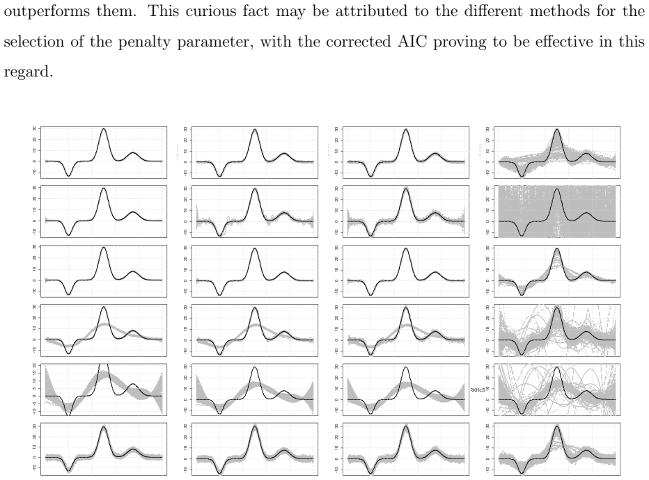
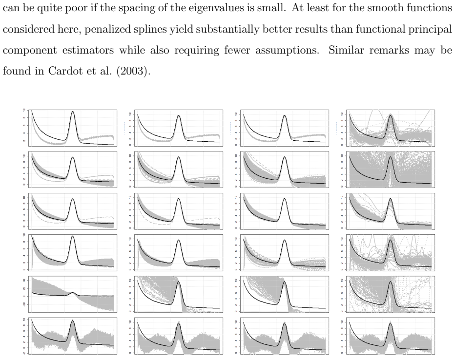
- [Table 1] For the closely-spaced case with beta3 and beta4, the reported mean errors for SSp and RKHS are very large even under Gaussian errors (e.g., 633.1, 686.5, 5823, 7737); this striking behavior is not commented on in the text and deserves an explanation or a caveat about the experimental setup.
- [Section 6] The term "redesceding M-estimators" appears to be a typo for "redescending M-estimators"; please correct it.
- [Section 3] The proof sketch in the main text is informative but the full proofs are deferred to a supplementary file; the authors should at least list the main lemmas or steps in the main text to allow readers to follow the argument without opening the supplement.
Circularity Check
No circularity: the rate theorems are derived from explicit design and smoothness assumptions, and no fitted constant enters the asymptotic rates.
full rationale
The paper's central claims, Theorem 1 and Corollary 1, are asymptotic rate statements of the form OP(K/n + K^{-2p} + lambda) for the penalized M-estimator. The proof, outlined in Section 3 and deferred to the technical supplement, is based on an asymptotic representation of the penalized M-estimator as the minimizer of a least-squares problem with pseudo-observations; this representation is an asymptotic expansion, not a restatement of the target rate. The terms K/n, K^{-2p}, and lambda arise from variance, spline approximation bias, and penalization bias respectively, and no fitted parameter is renamed as a prediction. The smoothing parameter lambda is allowed to tend to zero at any rate, and the corrected AIC in Section 2.2 is only used to select lambda in practice; it is not part of the theoretical rate derivation. Assumptions 1-5 and 6-9 are regularity, identifiability, and design-balance conditions rather than outputs of the method. There is no load-bearing self-citation chain and no definitional equivalence between input and result. One non-circular gap is worth noting: Assumption 4 requires psi in C^2, while Section 4.1 implements the Huber loss with c = 1.345, whose psi is only piecewise linear, so the stated theorem does not directly cover the default implementation; this is an assumption-to-implementation mismatch, not a circular dependence.
Assumptions & free parameters
free parameters (4)
- Huber tuning constant c =
1.345
- Spline basis dimension K =
40
- Penalty parameter lambda =
selected by corrected AIC
- Spline order p and penalty derivative q =
p = 4, q = 2
assumptions (5)
- domain assumption Assumption 1: functional predictors X are almost surely bounded in L2([0,1]).
- domain assumption Assumption 2: the true slope beta lies in a Holder class H^{p,v} with q < p.
- domain assumption Assumption 3: n^{-1}X^TX is nonsingular, permitting a singular limit.
- domain assumption Assumption 4: psi = rho' is C^2, with moment and identifiability conditions E psi(epsilon) = 0 and E psi'(epsilon) != 0.
- domain assumption Assumption 8: auxiliary scale sigma-hat satisfies sqrt(n)(sigma-hat - sigma) = O_P(1).
Cite this review
Pith. "Pith review of Robust penalized estimators for functional linear regression." pith.science (2026). https://pith.science/paper/T7733RHC
@misc{pith2026190808760,
  author       = {Pith},
  title        = {Pith review of: Robust penalized estimators for functional linear regression},
  year         = {2026},
  howpublished = {\url{https://pith.science/paper/T7733RHC}},
  note         = {Machine review of arXiv:1908.08760}
}
read the original abstract
Functional data analysis is a fast evolving branch of statistics. Estimation procedures for the popular functional linear model either suffer from lack of robustness or are computationally burdensome. To address these shortcomings, a flexible family of penalized lower-rank estimators based on a bounded loss function is proposed. The proposed class of estimators is shown to be consistent and can attain high rates of convergence with respect to prediction error under weak regularity conditions. These results can be generalized to higher dimensions under similar assumptions. The finite-sample performance of the proposed family of estimators is investigated by a Monte-Carlo study which shows that these estimators reach high efficiency while offering protection against outliers. The proposed estimators compare favorably to existing approaches robust as well as non-robust alternatives. The good performance of the method is also illustrated on a complex real dataset.
Figures

Figures from the paper (3 more)


Reference graph
Works this paper leans on
-
[1]
& Pascal, S.(1999) Functional linear model
Cardot, H., Ferraty, F. & Pascal, S.(1999) Functional linear model. Statistics & Probability Letters 45(1), 11–22
work page 1999
-
[2]
Cardot, H. , Ferraty, F. & Pascal, S.(2003) Spline estimators for the functional linear model. Statistica Sinica 13(3), 571–591
work page 2003
-
[3]
Claeksens, G., Krivobokova, T. & Opsomer, J. D. (2009) Asymptotic properties of penalised spline estimators. Biometrika 96(3), 529–544
work page 2009
-
[4]
& Pascal, S.(2009) Smoothing splines estimators for functional linear regression
Crambes, C., Kneip, A. & Pascal, S.(2009) Smoothing splines estimators for functional linear regression. The Annals of Statistics 37(1), 35–72
work page 2009
-
[5]
Crainiceanu, M. C. , Reiss, P. T. , Goldsmith, J., Huang, L., Huo, L., Scheipl, F., Greven, S., Harezlak, J., Kundu, M. G. & Zhao, Y. refund: Regression with functional data. CRAN. De Boor, C.(2001) A Practical Guide to Splines , revised edition. Springer
work page 2001
-
[6]
DeVore, R. A. & Lorentz, G. G.(1993) Constructive approximation. Springer. 30
work page 1993
-
[7]
Eubank, R. L. (1999) Nonparametric Regression and Spline Smoothing , second edition. CRC press
work page 1999
- [8]
Show all 48 references
-
[9]
& Varmuza, K.(2019) Multivariate Statistical Analysis in Chemometrics
Filzmoser, P. & Varmuza, K.(2019) Multivariate Statistical Analysis in Chemometrics. CRAN
2019
-
[10]
Goldsmith, J., Bobb, J., Crainiceanu, C. M. , Caffo, B. & Reich D.(2011) Pe- nalized functional regression. Journal of Computational and Graphical Statistics 20(4), 830–851
2011
-
[11]
& Scheipl, F.(2014) Estimator selection and combination in scalar-on- function regression
Goldsmith, J. & Scheipl, F.(2014) Estimator selection and combination in scalar-on- function regression. Computational Statistics & Data Analysis 70, 362–372
2014
-
[12]
Green, P. J. & Silverman, B. W. (1993) Nonparametric Regression and Generalized Linear Models: A roughness penalty approach . Chapman & Hall
1993
-
[13]
Springer
Gu, C.(2013) Smoothing spline ANOVA models, second edition. Springer
2013
-
[14]
& Horowitz, J
Hall, P. & Horowitz, J. L. (2007) Methodology and convergence rates for functional linear regression. The Annals of Statistics 35(1), 70–91
2007
-
[15]
Hampel, F. R. , Ronchetti, E. M. , Rousseeuw, P. J. & Stahel, W. A. (2011) Robust Statistics: The Approach Based on Influence Functions , second edition. Wiley. Horv´ath, L. & Kokoszka, P. (2012) Inference for functional data with applications . Springer. 31
2011
-
[16]
& Eubank, R
Hsing, T. & Eubank, R. L. (2015) Theoretical foundations of functional data analysis, with an introduction to linear operators . Wiley
2015
-
[17]
Huang, J., Horowitz, J. L. & Ma, S.(2008) Asymptotic properties of bridge estimators in sparse high-dimensional regression models. The Annals of Statistics 36(2), 587–613
2008
-
[18]
J.(1964) Robust Estimation of a Location Parameter
Huber, P. J.(1964) Robust Estimation of a Location Parameter. The Annals of Statistics 35(1), 73-101
1964
-
[19]
J.(1973) Robust Regression: Asymptotics, Conjectures and Monte Carlo
Huber, P. J.(1973) Robust Regression: Asymptotics, Conjectures and Monte Carlo. The Annals of Statistics 1(5), 799-821
1973
-
[20]
Huber, P. J. & Ronchetti, E. M.(2009) Robust Statistics, second edition. Wiley
2009
-
[21]
Hurvich, M. C. , Simonoff, J. & Tsai, C. (1998) Smoothing parameter selection in nonparametric regression using an improved Akaike information criterion. Journal of the Royal Statistical Society: Series B 60(2), 271–293
1998
-
[22]
James, G. M. , Wang, J. & Zhu, J. (2009) Functional linear regression that’s inter- pretable. The Annals of Statistics 37(5A), 271–293
2009
-
[23]
, Deraedt, I
Janssens, K. , Deraedt, I. , Schalm, O. & Veeckman, J. (1998) Composition of 15–17th century archaeological glass vessels excavated in Antwerp, Belgium . Springer
1998
-
[24]
Shi, P. & Li, G. (1995) Global convergence rates of B-spline M-estimators in nonpara- metric regression. Statistica Sinica 5(1), 303–318
1995
-
[25]
Journal of Multivariate Analysis 98(9), 1782–1804
Li, Y.& Hsing, T.(2007) On rates of convergence in functional linear regression. Journal of Multivariate Analysis 98(9), 1782–1804. 32
2007
-
[26]
A., Martin, D
Maronna, R. A., Martin, D. R. & Yohai, V. J.(2006) Robust Statistics: Theory and Methods. Wiley
2006
-
[27]
Maronna, R. A. & Yohai, V. J. (2013) Robust functional linear regression based on splines. Computational Statistics & Data Analysis 65, 46–55
2013
-
[28]
Morris, J. S. (2015) Functional regression Annual Review of Statistics and Its Applica- tions 2, 321–359
2015
-
[29]
Gijbels, I
Nagy, S. Gijbels, I. & Hlubinka, D.(2017) Depth-based recognition of shape outlying functions. Journal of Computational and Graphical Statistics 26(4), 883–893
2017
-
[30]
J.(2006) Numerical Optimization, second edition
Nocedal, J., & Weight, S. J.(2006) Numerical Optimization, second edition. Springer
2006
-
[31]
(2017) M-estimation for functional linear regression Communications in Statistics - Theory and Methods 46(8), 3782–3800
Qingguo, T. (2017) M-estimation for functional linear regression Communications in Statistics - Theory and Methods 46(8), 3782–3800. R Development Core Team (2019). R: A Language and Environment for Statistical Computing. Vienna, Austria: R Foundation for Statistical Computing...
2017
-
[32]
O.(1982) When the data are functions
Ramsay, J. O.(1982) When the data are functions. Psychometrika 47(4), 379–396
1982
-
[33]
Ramsay, J. O. & Dalzell, C. J. (1991) Some Tools for Functional Data Analysis. Journal of the Royal Statistical Society: Series B 53(3), 539–561
1991
-
[34]
Ramsay, J. O. & Silverman, B. W. (2005) Functional data analysis , second edition. Springer. 33
2005
-
[35]
Raymaekers, J., Rousseeuw, P. J. , Van den Bossche, W. & Hubert, M.(2019) Analyzing Data with Cellwise Outliers. CRAN
2019
-
[36]
Reiss, P. T. & Ogden, R. T.(2007) Functional principal component regression and func- tional partial least squares. Journal of the American Statistical Association 102(479), 984–996
2007
-
[37]
Reiss, P. T. , Goldsmith, J. , Shang, H. L. & Todd, R. T. (2017) Methods for scalar-on-function regression. International Statistical Review 85(2), 228–249
2017
-
[38]
Rousseeuw, P. J. & Yohai, V. J. (1984) Robust regression by means of S-estimators. Robust and nonlinear time series analysis , Springer
1984
-
[39]
Ruppert, D., Wand, M. P. & Carroll, R. J. (2003) Semiparametric Regression Cambridge
2003
-
[40]
Cambridge
Schumaker, L.(2007) Spline functions: basic theory , third edition. Cambridge
2007
-
[41]
& Lee, S
Shin, H. & Lee, S. (2016) An RKHS approach to robust functional linear regression. Statistica Sinica 26, 255–272
2016
-
[42]
J.(1985) Additive regression
Stone, C. J.(1985) Additive regression. The Annals of Statistics 13(2), 689–705
1985
-
[43]
Wahba, G.(1990) Spline models for observational data . Siam
1990
-
[44]
H.(1989) On M-processes and M-estimation
Welsh, A. H.(1989) On M-processes and M-estimation. The Annals of Statistics 17(1), 337–361
1989
-
[45]
Yohai, V. J. & Maronna, R. A. (1979) Asymptotic Behavior of M-Estimators for the Linear Model. The Annals of Statistics 7(2), 258–268. 34
1979
-
[46]
& Cai, T.(2010) A reproducing kernel Hilbert space approach to functional linear regression
Yuan, M. & Cai, T.(2010) A reproducing kernel Hilbert space approach to functional linear regression. The Annals of Statistics 38(6), 3412–3444
2010
-
[47]
, Ogden, T
Zhao, Y. , Ogden, T. R. & Reiss, P. T. (2012) Wavelet-based LASSO in functional linear regression. Journal of Computational and Graphical Statistics 21(3), 600–617
2012
-
[48]
& Chen, M.(2012) Spline estimators for semi-functional linear model
Zhou, J. & Chen, M.(2012) Spline estimators for semi-functional linear model. Statistics & Probability Letters 82(3), 505–513. 35
2012
Reviewed August 14, 2026 · model on record in the stance chip above.
Discussion (0). Continue with ORCID to comment.