REVIEW 4 major objections 6 minor 19 references
Imposing the Fundamental Dynamical Constraint of Hydrostatic Balance to Improve Global ML Weather Prediction
T0 review · 4 major / 6 minor · reviewed 2026-08-07 · deepseek-v4-flash
Pith's one-line read A soft constraint enforcing hydrostatic balance improves long-lead machine-learning weather forecasts, especially after 7-10 days.
desk verdict A clean physics-constrained ML weather idea with plausible skill gains, but the evaluation is not independent because the test years sit inside the validation period. read the letter →
The pith
A machine-rendered reading of the paper's core claim, the machinery that carries it, and where it could break.
The reading
What carries the argument
The load-bearing quantity is the layer residual $$ r_k = \frac{T_v(p_k)+T_v(p_{k-1})}{2} - \frac{g}{R}\ln\left(\frac{p_{k-1}}{p_k}\right)(Z_k - Z_{k-1}), $$ which measures, in temperature units, how far a pair of adjacent model levels sits from hydrostatic balance. The control mechanism is the error-tolerant loss $f(r_k) = (r_k/\alpha_k)^2/(1+e^{1-(r_k/\alpha_k)^2})$, which is nearly flat for $r_k \le \alpha_k$ and approaches a squared penalty for large $r_k$. The thresholds $\alpha_k$ are set from quantiles of the ERA5 imbalance distribution through the closed-form solution of the derivative-matching condition in Eq. (8), so the penalty is concentrated on the largest imbalances without fighting the small intrinsic imbalance in the data. The paper first tried a hard constraint that solved for upper-level temperatures from the hydrostatic relation, but error accumulation and coarse vertical resolution defeated it; the soft constraint is the mechanism that carries the results.
What would settle it
Repeat the q50 fine-tuning with the hydrostatic residual evaluated on the full 37-level ERA5 vertical grid instead of the six-level grid; if the 7-20 day RMSE improvement over the baseline disappears, the reported gains are an artifact of the coarse discretization, whereas if it persists, the constraint is capturing physical imbalance.
Extended reading notes
Core claim
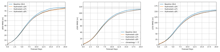
The core claim is that near-hydrostatic balance is a useful training penalty for long autoregressive forecasts even when the training data only approximately satisfy the balance. The paper defines a layer residual that measures, in temperature units, how far adjacent levels of geopotential height and virtual temperature sit from hydrostatic balance, and penalizes it with an error-tolerant loss that leaves small imbalances alone while strongly penalizing large ones. Fine-tuning the baseline with this loss yields, especially in the q50 variant, lower RMSE for geopotential heights at 850, 500, and 250 hPa and for wind-speed fields, with the gap over the baseline widening from about day 7 onward. In the hurricane Irma case, the constrained forecast removes a spurious wind maximum northwest of the eye that the baseline produces alongside a large virtual-temperature imbalance. The paper's interpretation is that single-step MSE is not the right target for long forecasts: what limits skill is the component of error that pushes the state out of balance, and the soft constraint reduces that component.
Load-bearing premise
The results rest on the assumption that the six-level hydrostatic residual, which is large and does not decrease during training in the upper layers, still measures the physical imbalance that degrades forecasts—so that penalizing it is what improves skill, rather than a numerical artifact of the coarse discretization.
Editorial extensions
If this is right
- If the claim is right, hydrostatic balance is a cheap general-purpose regularizer for ML weather models: adding it does not change the architecture, memory footprint, or inference cost.
- The best-performing constrained model crosses the 60-m RMSE threshold for 850-hPa geopotential height about one day later than the baseline, so the practical lead time of useful forecasts can be extended at these levels.
- Because the gains grow with lead time and are largest after 7-10 days, the constraint is most valuable for long-range and subseasonal prediction rather than for short-range skill.
- The constraint also improves physical consistency in extreme-event forecasts, as the Irma case shows, by suppressing an unbalanced spurious wind maximum near the eyewall.
Reading between the lines
- An extension the paper leaves implicit is to apply the same error-tolerant soft-constraint template to other balance relations, such as geostrophic balance or thermal wind, and test whether the gains combine or saturate.
- The paper's 'error orthogonal to the hydrostatic manifold' explanation is testable: one could compare spectral error-growth rates between the baseline and constrained models and check whether the constraint specifically damps the slowly growing balanced component of the error.
- Because the hydrostatic residual requires no extra data to compute, it could serve as a physicality diagnostic for other ML forecast or climate models, flagging when a roll-out begins to drift out of balance.
Editorial analysis
A structured set of objections, weighed in public.
Referee Report
Summary. The manuscript proposes to impose hydrostatic balance as a soft constraint on the DLWP/DLESyM global ML weather model. It defines a residual r_k from a discrete form of the hydrostatic relation (Eq. 7), penalizes it with an error-tolerant loss f(r_k) (Eq. 6), and finetunes a baseline model for three percentile thresholds p=0.5, 0.75, and 0.95. The authors report that the soft-constrained models have lower RMSE than the baseline for geopotential height and wind speed at 850, 500, and 250 hPa, especially beyond 7-10 days, and they present a qualitative case study of Hurricane Irma showing improved physicality. The paper also reports a failed hard-constraint implementation, a validation of the residual computation on an analytic profile (Appendix C), and a robustness experiment with different loss weights (Appendix B). The central claim is that imposing a dynamical constraint improves forecast skill without significant additional memory or scalability cost.
Significance. If the result held under an independent evaluation, it would be a useful demonstration that a physically motivated soft constraint improves the long-term autoregressive behavior of a coarse-resolution ML weather model at essentially no additional computational cost. The error-tolerant loss and the percentile-based calibration of alpha are clean, the discrete residual is validated in Appendix C, and the inclusion of a robustness experiment strengthens the paper. However, the empirical claim is not yet established because the evaluation period overlaps the validation period, the differences are not quantified with uncertainty estimates, and the causal attribution of the skill gains to the physical constraint is not fully supported by the training diagnostics.
major comments (4)
- [§3.1, §4, Appendix B] The test period is contained in the validation period. Section 3.1 states that 2016-2019 forms the validation set, and Section 4 evaluates forecasts on 2017 and 2018. Therefore the RMSE curves in Fig. 5 and the ACC statement in Section 4 are not independent of model-development decisions, including any early stopping, checkpoint selection, or the choice of p=0.5 as the best configuration. Appendix B's robustness check uses the same evaluation period and does not remedy this. The authors should evaluate on a truly held-out period (for example 2020-2021), or at least report model-selection and early-stopping rules that make no use of 2017-2018 data.
- [§4, Fig. 5] No uncertainty quantification accompanies the reported improvements. The RMSE curves for 2017-2018 are based on roughly 104 twice-weekly initializations and are temporally correlated. A claim such as 'substantial improvement beginning around 7 days' requires error bars, bootstrap confidence intervals, or an explicit paired significance test. Without those, the seven-to-ten-day differences in Fig. 5 may be within sampling variability. Please add such quantification and temper the quantitative claims accordingly.
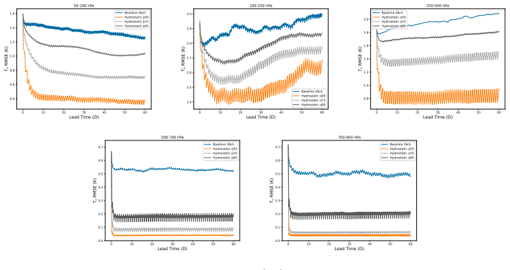
- [§3.2, §4] The causal attribution of the skill gains to hydrostatic balance is weakened by the manuscript's own observations. Fig. 4 shows that the validation loss for the hydrostatic residual does not decrease during training in the upper three layers, yet Fig. 5 reports substantial improvements at 250 hPa. This pattern suggests that fine-tuning may improve skill through generic effects such as continued training, learning-rate schedule, or altered loss landscape, rather than specifically through the physical constraint. A control experiment that fine-tunes the baseline with an equally weighted but non-physical residual, or with random targets, and evaluates on the same held-out period would help isolate the mechanism.
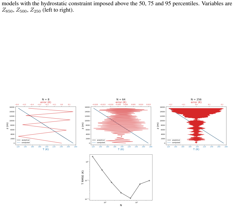
- [§2.3, Appendix C] The residual r_k in Eq. (7) is shown in Appendix C to be an accurate discretization of the hydrostatic relation on an idealized constant-lapse-rate profile, which is a good check. However, on real ERA5 data at the model's six-level resolution the upper-level imbalances remain large (Fig. 1b), and the training loss does not decrease there. Since the model still reports skill gains at 250 hPa, the physical interpretation of minimizing r_k is not yet fully supported. Please discuss, or better, test whether the coarse-grid r_k measures physical imbalance or a discretization artifact, for example by increasing the vertical resolution and checking whether the skill improvements and imbalance reductions scale together.
minor comments (6)
- [§3.1] The word 'hydrosatic' should be 'hydrostatic'.
- [§2.2] The phrase 'it's explicit computation' should be 'its explicit computation'.
- [§4] The word 'suprising' should be 'surprising', and the phrase 'in are clearly superior' appears to be missing a word.
- [Fig. 5] The label 'climatology * 2' is not defined; please state which climatological reference and period were used.
- [Tables 2 and 4] The notation alpha_k|Q(0.5) is confusing; please clarify what the vertical bar denotes.
- [General] The manuscript does not include a data and code availability statement; adding one would improve reproducibility.
Circularity Check
No circularity: the hydrostatic constraint is derived from the physical balance equation and evaluated as an empirical forecast-skill outcome; data-derived loss thresholds are hyperparameters, not renamed predictions.
full rationale
The paper's derivation chain is self-contained and not circular. Hydrostatic balance is introduced from the vertical momentum equation (Eq. 1), converted to a virtual-temperature form (Eq. 2), integrated to Eq. 4, and discretized as the residual rk in Eq. 7. The soft constraint loss in Eq. 6 penalizes this residual, and the alpha_k values in Eq. 9 are chosen from training-data quantiles Qk(p) via Eq. 8; they are loss-shaping parameters, not fitted forecasts of skill. The central claim — that finetuning with this constraint improves RMSE at 7–10 day lead times — is an empirical comparison of autoregressive forecasts shown in Fig. 5, not a quantity that is equal to the training loss or the residual by construction. The authors even report the opposite of a forced relationship: at 250 hPa the hydrostatic validation loss does not decrease during training, yet the constrained model shows improved forecast RMSE, which indicates the skill gain is an emergent rollout property rather than a restatement of the training objective. Self-citations to prior DLWP/ACE-style work ([6], [10]) concern network architecture and are not load-bearing for the hydrostatic-balance result. One legitimate statistical concern is that the 2017–2018 evaluation period lies inside the 2016–2019 validation set and only three p-quantile variants are compared, which could inflate the apparent q50 advantage; however, that is an evaluation-leakage/error-bar concern, not a circular reduction. No equation-level equivalence, renamed fit, or self-citation chain forces the reported improvement.
Assumptions & free parameters
free parameters (4)
- alpha_k (per vertical slab) =
Varies: e.g., 850-700 hPa alpha = 0.211 (q50), 0.475 (q75), 1.213 (q95); see Table 2
- Percentile p =
0.5, 0.75, 0.95 tested; q50 reported best
- Hydrostatic loss Lagrange multipliers =
1e-3 for lower slabs, 1e-4 for upper slabs (Appendix B uses 1e-4 for all)
- Prognostic variable loss weights =
Listed in Table 3
assumptions (5)
- domain assumption Hydrostatic balance is a valid leading-order approximation for synoptic-scale motions (horizontal scales > 20 km)
- standard math The trapezoidal/finite-difference discretization (4) is an accurate representation of the hydrostatic integral at six vertical levels
- domain assumption Virtual temperature approximation Tv = T(1 + 0.6078 q) captures moisture effects on density
- domain assumption Specific humidity is zero above 500 hPa
- domain assumption ERA5 reanalysis is an appropriate ground truth and baseline
Cite this review
Pith. "Pith review of Imposing the Fundamental Dynamical Constraint of Hydrostatic Balance to Improve Global ML Weather Prediction." pith.science (2026). https://pith.science/paper/TAJVKCTQ
@misc{pith2026250608285,
  author       = {Pith},
  title        = {Pith review of: Imposing the Fundamental Dynamical Constraint of Hydrostatic Balance to Improve Global ML Weather Prediction},
  year         = {2026},
  howpublished = {\url{https://pith.science/paper/TAJVKCTQ}},
  note         = {Machine review of arXiv:2506.08285}
}
read the original abstract
Forecasting weather accurately and efficiently is a critical capability in our ability to adapt to climate change. Data driven approaches to this problem have enjoyed much success recently providing forecasts with accuracy comparable to physics based numerical prediction models but at significantly reduced computational expense. However, these models typically do not incorporate any physics priors. In this work, we demonstrate improved skill of data driven weather prediction approaches by incorporating physical constraints, specifically in the context of the DLWP model (Karlbauer et. al. 2024). Near hydrostatic balance, between the vertical pressure gradient and gravity, is one of the most fundamental and well satisfied constraints on atmospheric motions. We impose this balance through both hard and soft constraints, and demonstrate that the soft constraint improves the RMSE of many forecast fields, particularly at lead times beyond 7-10 days. The positive influence of hydrostatic balance is also clearly evident in improving the physicality and strength of a 10-day forecast for hurricane Irma. These results show that adding appropriate physical constraints can improve the skill and fidelity of data driven weather models in a way that does not impose any significant additional memory capacity or scalability challenges.
Figures


Figures from the paper (6 more)



Reference graph
Works this paper leans on
-
[1]
Tom Beucler, Michael Pritchard, Stephan Rasp, Jordan Ott, Pierre Baldi, and Pierre Gentine. Enforcing Analytic Constraints in Neural Networks Emulating Physical Systems.Physical Review Letters, 126(9):098302, March 2021. Publisher: American Physical Society
work page 2021
-
[2]
Kaifeng Bi, Lingxi Xie, Hengheng Zhang, Xin Chen, Xiaotao Gu, and Qi Tian. Accurate medium-range global weather forecasting with 3D neural networks.Nature, 619(7970):533– 538, 2023
work page 2023
-
[3]
FengWu: Pushing the Skillful Global Medium-range Weather Forecast beyond 10 Days Lead
Kang Chen, Tao Han, Junchao Gong, Lei Bai, Fenghua Ling, Jing-Jia Luo, Xi Chen, Leiming Ma, Tianning Zhang, Rui Su, Yuanzheng Ci, Bin Li, Xiaokang Yang, and Wanli Ouyang. FengWu: Pushing the Skillful Global Medium-range Weather Forecast beyond 10 Days Lead. (arXiv:2304.02948), 2023
arXiv 2023
-
[4]
Lei Chen, Xiaohui Zhong, Feng Zhang, Yuan Cheng, Yinghui Xu, Yuan Qi, and Hao Li. FuXi: A cascade machine learning forecasting system for 15-day global weather forecast.npj Climate and Atmospheric Science, 6(1):1–11, 2023
work page 2023
-
[5]
On the lambert w function.Advances in Computational mathematics, 5:329–359, 1996
Robert M Corless, Gaston H Gonnet, David EG Hare, David J Jeffrey, and Donald E Knuth. On the lambert w function.Advances in Computational mathematics, 5:329–359, 1996
work page 1996
-
[6]
Espinosa, Raul Moreno, and Matthias Karlbauer
Nathaniel Cresswell-Clay, Bowen Liu, Dale Durran, Andy Liu, Zachary I. Espinosa, Raul Moreno, and Matthias Karlbauer. A Deep Learning Earth System Model for Stable and Efficient Simulation of the Current Climate. (arXiv:2409.16247), September 2024
arXiv 2024
-
[7]
K. M. Górski, E. Hivon, A. J. Banday, B. D. Wandelt, F. K. Hansen, M. Reinecke, and M. Bartelmann. HEALPix: A Framework for High-Resolution Discretization and Fast Analysis of Data Distributed on the Sphere.The Astrophysical Journal, 622(2):759, 2005
work page 2005
-
[8]
Hans Hersbach, Bill Bell, Paul Berrisford, Shoji Hirahara, András Horányi, Joaquín Muñoz- Sabater, Julien Nicolas, Carole Peubey, Raluca Radu, Dinand Schepers, et al. The era5 global reanalysis.Quarterly journal of the royal meteorological society, 146(730):1999–2049, 2020
work page 1999
Show all 19 references
-
[9]
Stable machine-learning parameter- ization of subgrid processes with real geography and full-physics emulation.arXiv preprint arXiv:2407.00124, 2024
Zeyuan Hu, Akshay Subramaniam, Zhiming Kuang, Jerry Lin, Sungduk Yu, Walter M Hannah, Noah D Brenowitz, Josh Romero, and Michael S Pritchard. Stable machine-learning parameter- ization of subgrid processes with real geography and full-physics emulation.arXiv preprint arXiv:240...
2024 arXiv
-
[10]
Durran, Raul A
Matthias Karlbauer, Nathaniel Cresswell-Clay, Dale R. Durran, Raul A. Moreno, Thorsten Kurth, Boris Bonev, Noah Brenowitz, and Martin V . Butz. Advancing Parsimonious Deep Learning Weather Prediction Using the HEALPix Mesh.Journal of Advances in Modeling Earth Systems, 16(8):e...
2024
-
[11]
Physics-informed machine learning: Case studies for weather and climate mod- elling.Philosophical transactions
Karthik Kashinath, M Mustafa, Adrian Albert, J.-L Wu, C Jiang, Soheil Esmaeilzadeh, Kamyar Azizzadenesheli, R Wang, Ashesh Chattopadhyay, A Singh, A Manepalli, D Chirila, R Yu, R Walters, B White, Heng Xiao, Hamdi Tchelepi, P Marcus, Animashree Anandkumar, and Mr Prabhat. Phys...
2021
-
[12]
Adam: A method for stochastic optimization.arXiv preprint arXiv:1412.6980, 2014
Diederik P Kingma. Adam: A method for stochastic optimization.arXiv preprint arXiv:1412.6980, 2014
2014 arXiv
-
[13]
Brenner, and Stephan Hoyer
Dmitrii Kochkov, Janni Yuval, Ian Langmore, Peter Norgaard, Jamie Smith, Griffin Mooers, James Lottes, Stephan Rasp, Peter Düben, Milan Klöwer, Sam Hatfield, Peter Battaglia, Alvaro Sanchez-Gonzalez, Matthew Willson, Michael P. Brenner, and Stephan Hoyer. Neural General Circul...
2023 arXiv
-
[14]
Learning skillful medium-range global weather forecasting
Remi Lam, Alvaro Sanchez-Gonzalez, Matthew Willson, Peter Wirnsberger, Meire Fortunato, Ferran Alet, Suman Ravuri, Timo Ewalds, Zach Eaton-Rosen, Weihua Hu, Alexander Merose, Stephan Hoyer, George Holland, Oriol Vinyals, Jacklynn Stott, Alexander Pritzel, Shakir Mohamed, and P...
2023
-
[15]
Simon Lang, Mihai Alexe, Matthew Chantry, Jesper Dramsch, Florian Pinault, Baudouin Raoult, Mariana C. A. Clare, Christian Lessig, Michael Maier-Gerber, Linus Magnusson, Zied Ben Bouallègue, Ana Prieto Nemesio, Peter D. Dueben, Andrew Brown, Florian Pappenberger, and Florence ...
2024
-
[16]
NVIDIA PhysicsNeMo: An open-source framework for physics- based deep learning in science and engineering, February 2023
PhysicsNeMo Contributors. NVIDIA PhysicsNeMo: An open-source framework for physics- based deep learning in science and engineering, February 2023
2023
-
[17]
Vallis.Atmospheric and Oceanic Fluid Dynamics
Geoffery K. Vallis.Atmospheric and Oceanic Fluid Dynamics. Cambridge University Press, second edition, 2017. 946 p
2017
-
[18]
Clark, Anna Kwa, W
Oliver Watt-Meyer, Brian Henn, Jeremy McGibbon, Spencer K. Clark, Anna Kwa, W. Andre Perkins, Elynn Wu, Lucas Harris, and Christopher S. Bretherton. ACE2: Accurately learning subseasonal to decadal atmospheric variability and forced responses, November 2024
2024
-
[19]
Climsim: A large multi-scale dataset for hybrid physics-ml climate emulation.Advances in Neural Information Processing Systems, 36:22070–22084, 2023
Sungduk Yu, Walter Hannah, Liran Peng, Jerry Lin, Mohamed Aziz Bhouri, Ritwik Gupta, Björn Lütjens, Justus C Will, Gunnar Behrens, Julius Busecke, et al. Climsim: A large multi-scale dataset for hybrid physics-ml climate emulation.Advances in Neural Information Processing Syst...
2023
Reviewed August 7, 2026 · model on record in the stance chip above.
Discussion (0). Sign in to comment.