REVIEW 5 major objections 5 minor 48 references
Synchronization transitions in spiking networks with adaptive coupling
T0 review · 5 major / 5 minor · reviewed 2026-08-06 · deepseek-v4-flash
Pith's one-line read In a ring of leaky integrate-and-fire neurons with Hebb-Oja adaptive couplings, slow weight evolution makes the network pass through chimera states of changing multiplicity and through bump states with different numbers of active domains…
desk verdict Novel adaptive-LIF result with a real gap between observation and interpretation; deserves review but needs the frozen-coupling comparison and ensemble statistics. read the letter →
The pith
A machine-rendered reading of the paper's core claim, the machinery that carries it, and where it could break.
The reading
What carries the argument
The load-bearing object is the time-dependent coupling matrix $\sigma_{jk}(t)$ with the Oja-normalized Hebbian rule $d\sigma_{jk}/dt = (1/\tau_\sigma)(u_j u_k - \alpha \, u_j u_j \, \sigma_{jk})$, which drives the mean effective coupling $\sigma_{\rm eff}(t)$ monotonically toward $c_u/\alpha$ while keeping the weights finite. The key control is $\tau_\sigma$, the ratio of the coupling-evolution timescale to the potential-evolution timescale. For $\tau_\sigma=1000$ the mean coupling sweeps slowly enough for the system to relax into each intermediate state; for $\tau_\sigma=2$ the sweep is too fast and the network lands directly in the asymptotic state. The Kuramoto order parameter $r(t)$ is the diagnostic that marks the transitions, especially the abrupt drop as $\sigma_{\rm eff}$ crosses zero.
What would settle it
Run the same LIF ring with the couplings frozen at the instantaneous mean effective value $\sigma_{\rm eff}(t)$ at each time and compare the spacetime plots and Kuramoto order parameter; if the adaptive trajectory's intermediate chimera multiplicities and bump configurations are not reproduced by the frozen runs with the same mean coupling, the claimed transitions between constant-coupling regimes are not established.
Extended reading notes
Core claim
The central claim is that an adaptive LIF network governed by the coupled potential and coupling equations crosses genuine synchronization regimes as the average effective coupling $\sigma_{\rm eff}(t)$ changes: starting from $\sigma_{\rm eff}=+2.1$ (bump regime) and ending at $\sigma_{\rm eff}=-0.7$ (chimera regime), the spacetime evolution shows a traveling bump state, then a drop in the Kuramoto order parameter near $\sigma_{\rm eff}=0$, then a two-headed chimera, a single-headed chimera, and finally a disorganized fluctuating phase; the reverse route from $-2.1$ to $+0.7$ passes from a two-headed chimera through incoherence to a one-headed chimera and then to two-bump and multi-bump states. The size and multiplicity of the coherent and incoherent, or active and subthreshold, domains change following $\sigma_{\rm eff}(t)$. The authors propose that slow adaptation acts like a continuation method, dragging the system through the states of the frozen-coupling system, whereas fast adaptation with $\tau_\sigma=2$ suppresses all intermediate states.
Load-bearing premise
The argument assumes that during slow coupling drift the network stays near the state that the constant-coupling system would have at the current mean effective coupling, even though the individual couplings are nonuniform and remember their history.
Editorial extensions
If this is right
- If the claim holds, chimera and bump states are not confined to networks with carefully tuned constant coupling; they appear as transient stages of a plastically adapting spiking network.
- Slow synaptic adaptation expands the repertoire of synchronization states the network can visit, while fast adaptation collapses that repertoire to the final asymptotic state.
- The route from positive to negative effective coupling is not the time-reverse of the route from negative to positive: the two directions pass through different sequences of chimera multiplicities and bump configurations.
- The Kuramoto order parameter provides a sharp, easily measurable marker of the crossing of zero effective coupling, which could be used to detect these transitions in simulation or experiment.
- The time needed to reach the asymptotic coupling state scales linearly with $\tau_\sigma$, so the duration of each intermediate synchronization regime can be controlled by adjusting the plasticity timescale.
Reading between the lines
- A direct test the authors did not report: freeze the couplings at the current mean effective value at each instant and compare the resulting spacetime pattern with the adaptive run; agreement would confirm the continuation picture, while disagreement would show that the nonuniform, history-dependent weights themselves create the observed multiplicities.
- If the continuation picture is right, the frozen-coupling phase diagram of the LIF ring could be used predictively: the sequence of chimeras and bumps should be readable from the trajectory of $\sigma_{\rm eff}(t)$ alone.
- The asymmetry between the two drift directions implies that an adaptive network's synchronization history is path-dependent; one could test this by reversing the sign of $c_u$ midway through a slow run and checking whether the state returns along a different sequence.
- The same slow-adaptation mechanism could be probed in other oscillator families, such as FitzHugh-Nagumo or Kuramoto networks, to see whether the traversal of hybrid states is generic or specific to integrate-and-fire dynamics.
Editorial analysis
A structured set of objections, weighed in public.
Referee Report
Summary. The manuscript studies a ring of N=1024 leaky integrate-and-fire neurons with nonlocal coupling (Eq. 3a) whose synaptic strengths evolve according to the Hebbian/Oja rule (Eq. 3c). It reports that when the weight dynamics are slow (large τσ, here 1000), the mean effective coupling σ_eff drifts monotonically from positive to negative (or vice versa), and the network is claimed to pass through chimera states with different numbers of incoherent domains and through bump states with different numbers of active and subthreshold domains; the size and multiplicity of these domains are said to follow the evolution of the average coupling strength. When the weight dynamics are fast (τσ = 2), these intermediate hybrid states are suppressed and the system quickly reaches its asymptotic state. The paper interprets the slow case as a kind of continuation process along the drifting coupling parameter.
Significance. If the central claim were established quantitatively, the paper would offer a useful demonstration that chimera and bump states can arise naturally during slow synaptic adaptation in a spiking network, rather than only under carefully prepared constant-coupling conditions. The qualitative observation of state changes in a single trajectory is suggestive, and the comparison between slow and fast adaptation time scales is conceptually interesting. However, the current evidence is based on single realizations and visual classification, the key adiabatic assumption is not tested, and the scalar mean coupling is not shown to be a sufficient descriptor of the nonuniform coupling matrix; the significance of the claimed transitions therefore remains unproven.
major comments (5)
- [Sec. VI (and Figs. 1-2)] The central interpretation that the adaptive network 'transits through' chimera regimes with different multiplicity relies on the unstated assumption that, during slow adaptation, the network remains close to the attractor of the constant-coupling system with the same instantaneous mean coupling. This continuation assumption is explicitly invoked in Sec. VI but never tested. I ask the authors to compare the adaptive trajectories against simulations of the frozen-coupling system with uniform σ_eff equal to the instantaneous mean from Eq. (5b) at matching times. Without such a comparison, the observed spacetime patterns could be adaptive transients unique to the time-varying coupled system, and the phrase 'transits through' is not supported.
- [Sec. III, Figs. 1-2] Every scenario description is based on a single realization starting from one draw of random initial potentials; no ensemble statistics, standard deviations, or error bars are provided. The claims that the number and size of coherent/incoherent domains 'follow' the average coupling strength (Abstract, Sec. III) require quantitative definitions of domain multiplicity and domain boundaries, such as a local Kuramoto order parameter with a threshold or firing-rate-based criteria, applied over many initial conditions. As presented, the trajectory-level narrative is anecdotal and cannot support the general quantitative claim.
- [Abstract (and Sec. IV)] The time-scale condition is stated backwards in the abstract: the paper's slow-adaptation regime corresponds to large τσ = 1000 (Sec. IV), where the link dynamics are slower than the potential dynamics, yet the abstract says transitions occur 'provided that the time scales governing the link dynamics are relatively small compared to the time scales of the potential evolution.' This contradicts the model setup and should be corrected to refer to slow (large-τσ) link evolution; the claim as written would falsely predict transitions only in the fast-adaptation case.
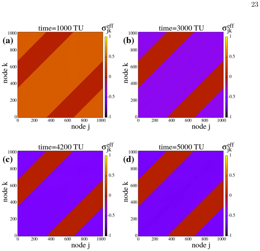
- [Sec. V B, Figs. 8-9] Figures 8-9 show that the coupling matrix is strongly nonuniform and history-dependent, with broad distributions of σ_eff values during the chimera-to-bump transition. This undermines the use of the scalar mean σ_eff(t) (Eq. 5b) as the state descriptor that controls the observed chimera multiplicity. The paper should either demonstrate that the dynamics depend on the mean alone (e.g., by comparing against a system with uniform but time-varying coupling at the same mean), or replace the scalar 'following' statement with a more precise description that accounts for the distribution width and spatial structure of the couplings.
- [Sec. II (numerical methods)] The manuscript does not report the numerical integrator, time step, event-detection method for the reset condition (Eq. 3b), or the scheme used to integrate the stiff coupling equation (Eq. 3c). Because the model is event-driven, the discretization and the handling of simultaneous or near-simultaneous threshold crossings can affect whether chimera and bump transients appear. The authors should describe the algorithm in sufficient detail and, ideally, provide code or data to support reproducibility; the current 'data available upon request' statement is not enough for a computational study.
minor comments (5)
- [Sec. II C, Eq. (7)] The phase definition θ_j = 2π u_j / u_th is introduced without explanation; please clarify that it is a linear rescaling of the potential used for the Kuramoto order parameter and is not the natural phase of the LIF oscillator, and note how this choice affects r values near reset.
- [Sec. IV, Fig. 5] The linear fit τ_steady = A τσ + B with A = 6.4, B = 5.3 is presented as empirical, and the claim that B should vanish is argued from τσ = 0. Since the data have a quoted error of ±10, this consistency check is fine, but it should be phrased as a compatibility statement rather than a derivation.
- [Abstract] The first sentence 'Adaptive link sizes is a major breakthrough step in evolving networks' is awkwardly phrased and contains a grammatical error; please revise for clarity.
- [Sec. V A] In the description of Fig. 6, the sentence 'the uncoupled connections are all colored brown-red' refers to zero-weight entries; please clarify that the color scale includes σ_eff = 0 and that this component of the matrix is time-invariant.
- [References] References [17] and [19] both list the article number 033146 (Entropy 35 and Chaos 35, respectively); please verify that these are correct and not a typographical duplication.
Circularity Check
No significant circularity: the adaptive-transition observations are direct simulations of Eqs. (3), and the only fitted relation is a peripheral empirical scaling law.
full rationale
The central claims are numerical observations of Eqs. (3), not consequences of a fitted parameter. The average coupling strength σeff(t) is defined by Eq. (5) as the population mean of the adaptive weights, and the statement that chimera and bump multiplicities follow σeff(t) is a reported correlation from spacetime plots and the Kuramoto order parameter (Figs. 1-2), not a quantity defined to equal the target. The only explicit fit, τsteady state = A τσ + B in Fig. 5, is presented as an empirical scaling law for relaxation to the Oja steady state; its parameters are acknowledged to depend on tolerance ϵ and system parameters, and it is not used to predict the chimera or bump transitions. Prior work by the same authors is cited to identify constant-coupling regimes of LIF networks (e.g., Refs. [14,15,18,20,45,46,48]), but these citations are background labeling, not load-bearing: the adaptive runs are initialized and interpreted using those regimes, while the intermediate states are read off the simulations themselves. No uniqueness theorem is imported, and no ansatz is smuggled in via citation; the Oja rule is taken from external references [30,31]. The continuation remark in Sec. VI is explicitly an analogy, not a derivation, and the paper does not claim to prove an adiabatic theorem. The absence of a timescale-separation check or comparison with the frozen-coupling phase diagram is a completeness and evidence limitation of the interpretation, but it does not make any step circular, because nothing in the derivation is equivalent by construction to the reported transitions. The abstract contains a likely reversed timescale phrase (relatively small instead of relatively large), but that is an internal wording inconsistency, not a circular argument.
Assumptions & free parameters
free parameters (5)
- alpha (Oja forgetting constant) =
1.0
- cu (effective coupling control parameter) =
-0.7 and +0.7
- initial coupling strength sigma_jk(0) =
-3.0
- tau_sigma (adaptation time scale) =
1000 (slow) and 2 (fast)
- linear fit coefficients A and B =
A=6.4, B=5.3
assumptions (5)
- domain assumption The LIF neuron with instantaneous reset at threshold is a valid model of spiking dynamics.
- domain assumption Hebbian plasticity can be represented as dsigma_jk/dt proportional to u_j u_k minus alpha u_j u_j sigma_jk, using instantaneous potentials rather than firing rates.
- domain assumption Nonlocal diffusive coupling with symmetric range R approximates gap-junction coupling.
- ad hoc to paper During slow adaptation, the network remains close to the attractors of the frozen-coupling system for the current average coupling (continuation assumption).
- domain assumption Random uniform initial potentials and homogeneous initial couplings represent generic initial conditions.
Cite this review
Pith. "Pith review of Synchronization transitions in spiking networks with adaptive coupling." pith.science (2026). https://pith.science/paper/TC2CCSUV
@misc{pith2026250717443,
  author       = {Pith},
  title        = {Pith review of: Synchronization transitions in spiking networks with adaptive coupling},
  year         = {2026},
  howpublished = {\url{https://pith.science/paper/TC2CCSUV}},
  note         = {Machine review of arXiv:2507.17443}
}
read the original abstract
Adaptive link sizes is a major breakthrough step in evolving networks and is now considered as an essential process both in biological and artificial neural networks. In adaptive networks the link weights change in time and, in brain dynamics, these changes are controlled by the potential variations of the pre- and post-synaptic neurons. In particular, in biological neural networks the adaptivity of the links (synapses) was first addressed by D. Hebb who proposed the rule that neurons which fire together wire together. In the present study, we explore the effects of adaptive linking in networks where hybrid synchronization patterns (solitaries, chimeras and bump states) are observed in the absence of adaptivity (i.e., for constant coupling strengths). The network consists of Leaky Integrate-and-Fire (LIF) neurons coupled nonlocally in a 1D ring geometry. The adaptivity follows the Hebbian principle adjusted by the Oja rule to avoid unbounded increase of the coupling strengths. Our results indicate that, for negative coupling strengths, the adaptive LIF network may transit through chimera state regimes with different multiplicity, provided that the time scales governing the link dynamics are relatively small compared to the time scales of the potential evolution. Moreover, the size of the coherent and incoherent domains of the chimera and their multiplicity change following the average coupling strength in the network. Similar results are shown for the case of bump states: for positive coupling strengths, the adaptive LIF network transits through states of different number of active and subthreshold domains. The size and number of these domains also follow the evolution of the average coupling strength. Such transient effects are suppressed when the time scales governing the link adaptive dynamics become of the same order as the time scales governing the potential dynamics.
Figures


Figures from the paper (7 more)




Reference graph
Works this paper leans on
-
[1]
M. I. Rabinovich, P. Varona, A. I. Selverston, and H. D. I. Abarbanel, Reviews of Modern Physics 78, 1213 (2006)
work page 2006
-
[2]
Berner, T
R. Berner, T. Gross, C. Kuehn, J. Kurths, and S. Yanchuk, Physics Reports 1031, 1 (2023)
2023
-
[3]
D. O. Hebb, The organization of behavior: A neuropsychological theory (John Willey and Sons, Inc, New York, 1949)
work page 1949
-
[4]
Y. Kuramoto and D. Battogtokh, Nonlinear Phenomena in Complex Systems 5, 380 (2002)
work page 2002
-
[5]
D. M. Abrams and S. H. Strogatz, Physical Review Letters 93, 174102 (2004). 30
work page 2004
-
[6]
O. E. Omel’chenko, Nonlinearity 31, R121 (2018)
work page 2018
-
[7]
I. Omelchenko, O. E. Omel’chenko, P. H¨ ovel, and E. Sch¨ oll, Physical Review Letters 110, 224101 (2013)
work page 2013
-
[8]
I. Omelchenko, A. Provata, J. Hizanidis, E. Sch¨ oll, and P. H¨ ovel, Physical Review E 91, 022917 (2015)
work page 2015
Show all 48 references
-
[9]
Hizanidis, V
J. Hizanidis, V. Kanas, A. Bezerianos, and T. Bountis, International Journal of Bifurcations and Chaos 24, 1450030 (2014)
2014
-
[10]
Ulonska, I
S. Ulonska, I. Omelchenko, A. Zakharova, and E. Sch¨ oll, Chaos 26, 094825 (2016)
2016
-
[11]
E. N. Nganso, S. N. Mbouna, R. Yamapi, G. Filatrella, and J. Kurths, Chaos, Solitons & Fractals 169, 113235 (2023)
2023
-
[12]
C. R. Laing and C. C. Chow, Neural Computations 13, 1473 (2001)
2001
-
[13]
O. E. Omel’chenko and C. R. Laing, Physical Review E 110, 034411 (2024)
2024
-
[14]
N. D. Tsigkri-DeSmedt, J. Hizanidis, P. H¨ ovel, and A. Provata, European Physical Journal - Special Topics 225, 1149 (2016)
2016
-
[15]
N. D. Tsigkri-DeSmedt, J. Hizanidis, E. Sch¨ oll, P. H¨ ovel, and A. Provata, The European Physical Journal B 90, 139 (2017)
2017
-
[16]
Avitabile, J
D. Avitabile, J. L. Davis, and K. Wedgwood, SIAM Review 65, 147 (2023)
2023
-
[17]
Provata, Y
A. Provata, Y. Almirantis, and W. Li, Entropy 35, 033146 (2025)
2025
-
[18]
Schmidt, T
A. Schmidt, T. Kasimatis, J. Hizanidis, A. Provata, and P. H¨ ovel, Physical Review E 95, 032224 (2017)
2017
-
[19]
Provata, J
A. Provata, J. Hizanidis, K. Anesiadis, and O. Omel’chenko, Chaos 35, 033146 (2025)
2025
-
[20]
Kasimatis, J
T. Kasimatis, J. Hizanidis, and A. Provata, Physical Review E 97, 052213 (2018)
2018
-
[21]
Tamaki, J
M. Tamaki, J. W. Bang, T. Watanabe, and Y. Sasaki, Current Biology 26, 1190 (2016)
2016
-
[22]
N. C. Rattenborg, Naturwissenschaften 93, 413 (2006)
2006
-
[23]
N. C. Rattenborg, C. J. Amlaner, and S. L. Lima, Neuroscience and Biobehavioral Reviews 24, 817 (2000)
2000
-
[24]
Ramlow, J
L. Ramlow, J. Sawicki, A. Zakharova, J. Hlinka, J. C. Claussen, and E. Sch¨ oll, Europhysics Letters 126, 50007 (2019)
2019
-
[25]
R. C. Gutierrez, A. Amann, S. Assenza, J. Gomez-Gardenes, V. Latora, and S. Boccaletti, Physical Review Letters 107, 234103 (2011)
2011
-
[26]
Aoki and T
T. Aoki and T. Aoyagi, Physical Review E 84, 066109 (2011). 31
2011
-
[27]
D. V. Kasatkin, S. Yanchuk, E. Schoell, and V. Nekorkin, Physical Review E 96, 062211 (2017)
2017
-
[28]
V. K. Chandrasekar, J. H. Sheeba, B. Subash, M. Lakshmanan, and J. Kurths, Physica D 267, 36 (2014)
2014
-
[29]
S. Huo, C. Tian, L. Kang, and Z. Liu, Nonlinear Dynamics 96, 75 (2019)
2019
-
[30]
Oja, Journal of Mathematical Biology 15, 267 (1982)
E. Oja, Journal of Mathematical Biology 15, 267 (1982)
1982
-
[31]
Oja, International Journal of Neural Systems 1, 61 (1989)
E. Oja, International Journal of Neural Systems 1, 61 (1989)
1989
-
[32]
L. M. Lapique, J. Physiol. Pathol. G´ en´ erale9, 567 (1907)
1907
-
[33]
L. F. Abbott, Brain Research Bulletin 50, 303 (1999)
1999
-
[34]
Brunel and M
N. Brunel and M. C. W. van Rossum, Biological Cybernetics 97, 337 (2007)
2007
-
[35]
A. N. Burkitt, Biological Cybernetics 95, 1 (2006)
2006
-
[36]
M. S. Santos, P. R. Protachevicz, K. C. Iarosz, I. L. Caldas, R. L. Viana, F. S. Borges, H. P. Ren, J. D. Szezech, A. M. Batista, and C. Grebogi, Chaos 29, 043106 (2019)
2019
-
[37]
Luccioli and A
S. Luccioli and A. Politi, Physical Review Letters 105, 158104 (2010)
2010
-
[38]
S. Olmi, A. Politi, and A. Torcini, Europhysics Letters 92, 60007 (2010)
2010
-
[39]
Olmi, , and A
S. Olmi, , and A. Torcini, in Nonlinear Dynamics in Computational Neuroscience , edited by F. Corinto and A. Torcini (PoliTo Springer Series, Cham, Switzerland, 2019) Chap. 5, pp. 65–79
2019
-
[40]
Politi and M
A. Politi and M. Rosenblum, Physical Review E 91, 042916 (2015)
2015
-
[41]
Politi, E
A. Politi, E. Ullner, and A. Torcini, European Physical Journal: Special Topics 227, 1185 (2018)
2018
-
[42]
Ullner, A
E. Ullner, A. Politi, and A. Torcini, Physical Review Research 2, 023103 (2020)
2020
-
[43]
Gerstner and W
W. Gerstner and W. M. Kistler, Spiking neuron models: Single neurons, populations, plasticity (Cambridge University Press, Cambridge, 2002)
2002
-
[44]
Ermentrout, Reports of Progress in Physics 61, 353 (1998)
B. Ermentrout, Reports of Progress in Physics 61, 353 (1998)
1998
-
[45]
S. Olmi, S. Petkoski, M. Guye, F. Bartolomei, and V. Jirsa, PLoS Computational Biology 15, e1006805 (2019)
2019
-
[46]
Provata, Journal of Physics: Complexity 5, 025011 (2024)
A. Provata, Journal of Physics: Complexity 5, 025011 (2024)
2024
-
[47]
S. H. Strogatz, Physica D 143, 1 (2000)
2000
-
[48]
N. D. Tsigkri-DeSmedt, I. Koulierakis, G. Karakos, and A. Provata, The European Physical Journal B 91, 305 (2018)
2018
Reviewed August 6, 2026 · model on record in the stance chip above.
Discussion (0). Continue with ORCID to comment.