Forecasting age distribution of death counts: An application to annuity pricing

Han Lin Shang; Steven Haberman

REVIEW 3 major objections 5 minor 4 references

Forecasting age distribution of death counts: An application to annuity pricing

T0 review · 3 major / 5 minor · reviewed 2026-08-14 · deepseek-v4-flash

Challenge this review Re-run · record.json Download PDF Read on arXiv ↗ Review JSON

Pith's one-line read Modelling age-specific life-table death counts as compositional data yields more accurate one- to 20-year-ahead forecasts of the death distribution and improves temporary annuity prices.

desk verdict A useful CoDa extension whose headline comparison is undermined by test-set selection of L=6. read the letter →

arxiv 1908.01446 v1 pith:TF7463D6 submitted 2019-08-05 stat.AP stat.ME

Han Lin Shang , Steven Haberman This is my paper · ORCID

classification stat.APstat.ME

keywords compositionaldataanalysislife-tabledeathcountslog-ratiotransformationprincipalcomponentmortalityforecastingtemporaryannuitypricingbootstrappredictionintervalsLee-Cartermethod

verification ladder T0 review T1 audit T2 compute T3 formal

The pith

A machine-rendered reading of the paper's core claim, the machinery that carries it, and where it could break.

The reading

This paper argues that the age distribution of life-table death counts should be forecast as compositional data: vectors of age-specific death counts that must sum to a fixed radix, transformed into unconstrained coordinates before forecasting. On Australian female and male life-table death counts from 1921 to 2014, the paper claims this approach, using principal component analysis with an automatic exponential-smoothing forecast of the component scores and retaining six components, gives more accurate one- to 20-step-ahead point and interval forecasts than the Lee-Carter, Hyndman-Ullah, and two random-walk benchmarks. The improved death-count forecasts feed directly into survival probabilities, and the paper shows they produce single-premium temporary annuity prices with bootstrap prediction intervals for ages 60 to 105 and maturities up to 30 years. A demographer or actuary who trusts the comparison would adopt the method for mortality forecasting and annuity pricing.

What carries the argument

The central object is the vector of age-specific life-table death counts, treated as compositional data in the simplex: $K$ positive components summing to the life-table radix, here 100,000. The machinery is the centred log-ratio transformation $z_{t,x}=\ln(f_{t,x}/g_t)$, where $f_{t,x}$ is the de-centred proportion and $g_t$ the geometric mean over ages, followed by principal component analysis of the transformed matrix, automatic ETS forecasting of the resulting principal component scores, and inverse transformation back to death-count space. The paper also builds interval forecasts by bootstrapping $h$-step-ahead score forecast errors and model residuals. Choosing $L=6$ principal components rather than the one or two selected by cumulative variance is what the forecast comparison shows to be most accurate.

What would settle it

Re-run the expanding-window forecast comparison with Lee-Carter and Hyndman-Ullah converted to death counts using the exact life-table identity $q_x = m_x / (1 + (1-a_x)m_x)$ (or a direct estimate of $q_x$) instead of the exponential approximation, and compare high-age errors separately; if CoDa's advantage over these benchmarks shrinks or reverses at ages above about 80, the reported superiority is an artifact of the conversion.

Watch

Extended reading notes

Core claim

The central claim is that forecasting the distribution of life-table deaths in its natural constrained sample space beats forecasting mortality rates and converting. The method models the relative proportions $d_{t,x}/\sum_x d_{t,x}$, applies a centred log-ratio transformation to break the sum constraint, estimates principal components and scores, forecasts each score with an ETS model selected automatically, then back-transforms and rescales to the 100,000 radix. With $L=6$ components and ETS, the paper reports the smallest MAPE and mean interval score among the CoDa, Hyndman-Ullah, Lee-Carter, and random-walk-with/without-drift methods, with the gap typically widening at longer horizons. It also proposes a nonparametric bootstrap that resamples multi-step score forecast errors and model residuals to build prediction intervals for death counts, survival probabilities, and annuity prices. The conclusion is that CoDa with ETS and $L=6$ is the recommended method for forecasting the age distribution of death counts and for pricing temporary immediate annuities.

Load-bearing premise

The load-bearing premise is that converting Lee-Carter and Hyndman-Ullah mortality-rate forecasts to death counts via $q_x = 1 - e^{-m_x}$ is a fair implementation of those benchmarks; the paper itself notes this approximation may explain their poorer performance at high ages, so if it biases the benchmarks downward, the CoDa method's superiority would be partly an artifact.

Editorial extensions

If this is right

If the central claim holds, demographers can derive survival probabilities and life expectancy directly from death-count forecasts that respect the radix constraint, avoiding inconsistencies from separately forecast mortality rates.
Actuaries can price temporary immediate annuities with point estimates and 95% prediction intervals; the paper's tables show prices for ages 60 to 105 and maturities 5 to 30 at a 3% interest rate.
The CoDa method's advantage grows with forecast horizon, so it is most valuable for long-term contracts, which the paper notes become almost lifetime annuities at high entry ages.
Because the method allows the rate of mortality improvement to vary over time, it captures shifts in the age-at-death distribution that fixed-coefficient Lee-Carter extrapolations miss.
The proposed bootstrap interval construction outperforms the existing CoDa bootstrap of Bergeron-Boucher et al. (2017) in the reported interval-score comparisons.

Reading between the lines

Editorial extensions of the paper, not claims the author makes directly.

A testable extension is to repeat the comparison on other countries in the Human Mortality Database; if the CoDa-ETS-$L=6$ advantage is not universal, the recommendation should be qualified by mortality regime.
The comparison's dependence on the $q_x=1-e^{-m_x}$ conversion for Lee-Carter and Hyndman-Ullah suggests that a head-to-head using exact life-table conversion could narrow the gap; until then, the claimed superiority at high ages should be read cautiously.
Because compositional forecasts automatically enforce positivity and summation, they may be especially useful for small populations or subpopulations where benchmark methods produce implausible negative or non-integer death counts.
The same log-ratio machinery could be applied to other constrained demographic distributions, such as cause-of-death composition or migration age profiles, with analogous forecasting and interval-score comparisons.

Share X Bluesky LinkedIn Reddit HN

Signed reviews

No signed human review yet.

Editorial analysis

A structured set of objections, weighed in public.

Desk editor's note, referee report, and a circularity audit.

Desk Editor's Note

read the letter

Hi [Colleague],

Quick take: this is a competent applied extension of compositional data analysis to mortality forecasting, with a real chance of being useful, but the headline result is weaker than it looks because the recommended L=6 is selected on the same holdout that is later used to claim superiority. That is not a fatal flaw, but it is exactly the kind of test-set tuning that inflates apparent out-of-sample performance, and the paper does not report any separate validation or nested model selection.

What is actually new: Oeppen (2008) and Bergeron-Boucher et al. (2017) introduced CoDa for life-table death counts with a single component (or somewhat limited component choice). Here the authors allow multiple principal components, use the automatic ETS search of Hyndman and Khandakar (2008) to forecast scores, propose a bootstrap interval scheme that samples both forecast errors and model residuals, and demonstrate the method on temporary annuity pricing. The empirical comparison on Australian data (1921-2014) is not in the prior work, and the annuity application is a natural and useful extension. The paper also shares R code and data, which is appreciated.

The main soft spot is the L selection. In Section 3.1, L is chosen by CPV (L=1 for females, L=2 for males). Section 5.2 then says L=6 'generally provides more accurate' errors, and the conclusion recommends it. But the evidence for L=6 comes from the same expanding-window holdout that produced Table 1. So the reported MAPE and interval scores for the recommended configuration are not independent; they are in-sample relative to model selection. The margin over HU and LC could shrink under a fairer protocol. This is fixable: use the first part of the data to choose L, then evaluate on the rest, or use nested CV. I'd ask the authors to do that before accepting the headline claim.

Secondary issues: the paper does not report empirical coverage of the bootstrap intervals, only interval scores; coverage would reassure that the proposed interval method is not just sharp but calibrated. The single-country design limits generalizability, though that is common in this literature. The q=1-exp(-m) conversion for LC/HU is acknowledged by the authors as a possible reason for their poorer performance at high ages; it is a standard approximation, so it is not damning, but it is one more reason to be cautious about the magnitude of the claimed superiority.

Overall, the paper is worth a serious referee. The method is promising, the writing is clear, and the application is relevant. But the L-selection issue needs to be addressed before the main claim can be taken at face value. I would send it to review with a request for nested validation or a separate tuning period, and for a coverage analysis of the intervals.

Best, [You]

Referee Report

3 major / 5 minor

Summary. The paper proposes a compositional data analysis (CoDa) approach for forecasting the age distribution of life-table death counts. Using Australian sex-specific period life-table death counts from 1921 to 2014, the method applies a centred log-ratio transformation, principal component analysis, and exponential smoothing (ETS) forecasts of principal component scores, with bootstrap prediction intervals. The authors compare point and interval forecast accuracy against the Lee-Carter method, the Hyndman-Ullah method, and random-walk benchmarks in an expanding-window holdout evaluation, and then use the forecasts to price single-premium temporary immediate annuities. The central claim is that CoDa with ETS and L=6 principal components outperforms the benchmarks for one- to 20-step-ahead forecasts.

Significance. If the comparative claim holds, the paper offers a useful and practical extension of compositional-data mortality forecasting: it adapts the Hyndman-Ullah functional-data approach to the constrained space of life-table death counts, adds a bootstrap interval procedure, and connects improved death-count forecasts to annuity pricing. The strengths are the use of public HMD data, standard evaluation criteria (MAPE and Gneiting-Raftery interval scores), a clear actuarial application, and the provision of R code and data files. The main weakness is that the recommended configuration (L=6, ETS) is selected by inspecting the same holdout sample that is later used to establish superiority, which undermines the independence of the headline out-of-sample comparison. The benchmark conversion from mortality rates to death counts is also a plausible source of unfair disadvantage to Lee-Carter and Hyndman-Ullah.

major comments (3)

[Sections 5.1 and 5.2; Table 1] The recommended configuration L=6 is selected on the same expanding-window holdout used to report forecast superiority. Section 3.1 states that the cumulative-percentage-of-variance criterion selects L=1 for females and L=2 for males; Section 5.2 then recommends L=6 because it 'generally provides more accurate point and interval forecast accuracies' than the CPV-selected choices, based on Table 1. Since Table 1 is computed from the same holdout used to support the abstract's 'outperforms' claim, the reported error metrics for CoDa-ETS(L=6) are not independent test-set results. The authors should either use a separate validation period for model selection, implement nested cross-validation, or at minimum report the comparison both for the CPV-selected L and for the sensitivity L=6 while clearly flagging which numbers are selection-influenced. Without this, the size of the reported improvement over Hyndman-Ullah and Lee-Carter may be inflated by test-set tuning.
[Sections 3.3.1 and 5.2] The comparison may unfairly disadvantage the Lee-Carter and Hyndman-Ullah benchmarks through the conversion of forecast central mortality rates to death counts using q = 1 - exp(-m). As the paper itself acknowledges in Section 5.2, this approximation is likely to be poor at high ages, and the authors suggest it may explain the benchmarks' worse performance. Because the central claim is improved forecast accuracy over these benchmarks, the conversion assumption is load-bearing. The authors should use the exact life-table relation available from HMD (or an approximation with an explicit separation factor) and quantify how sensitive the rankings in Table 1 are to this choice. If the conversion is retained, a sensitivity analysis comparing alternative conversions is needed to establish that the CoDa advantage is not an artifact of the benchmark implementation.
[Sections 3.2 and 5.1; Tables 1 and 3] Interval forecast performance is assessed only through the interval score, with no empirical coverage check for the proposed bootstrap prediction intervals. The interval score rewards narrow intervals but does not, by itself, reveal systematic under- or over-coverage; Table 3 shows very narrow 95% intervals for annuity prices, and it is unclear whether nominal 80% and 95% coverage are achieved in the holdout. The authors should report empirical coverage rates alongside interval scores. In addition, the MAPE and interval-score differences between methods are reported as point values without any measure of uncertainty (e.g., standard errors or Diebold-Mariano-type tests), so the statistical significance of the claimed superiority is not established.

minor comments (5)

[Supplementary Tables 4 and 5] The column headings 'K = 6' should read 'L = 6' for consistency with the main text's notation for the number of principal components.
[Section 3.1, item on log-ratio transformations] The term 'multiple log-ratio' appears to be a typo for 'multiplicative log-ratio'; please correct it.
[Section 6 and Tables 2-5] The text in Section 6 refers to 'Table 4' and 'Table 5' for female annuity prices, but the tables in the main text are numbered 2 and 3; the table numbering should be made consistent.
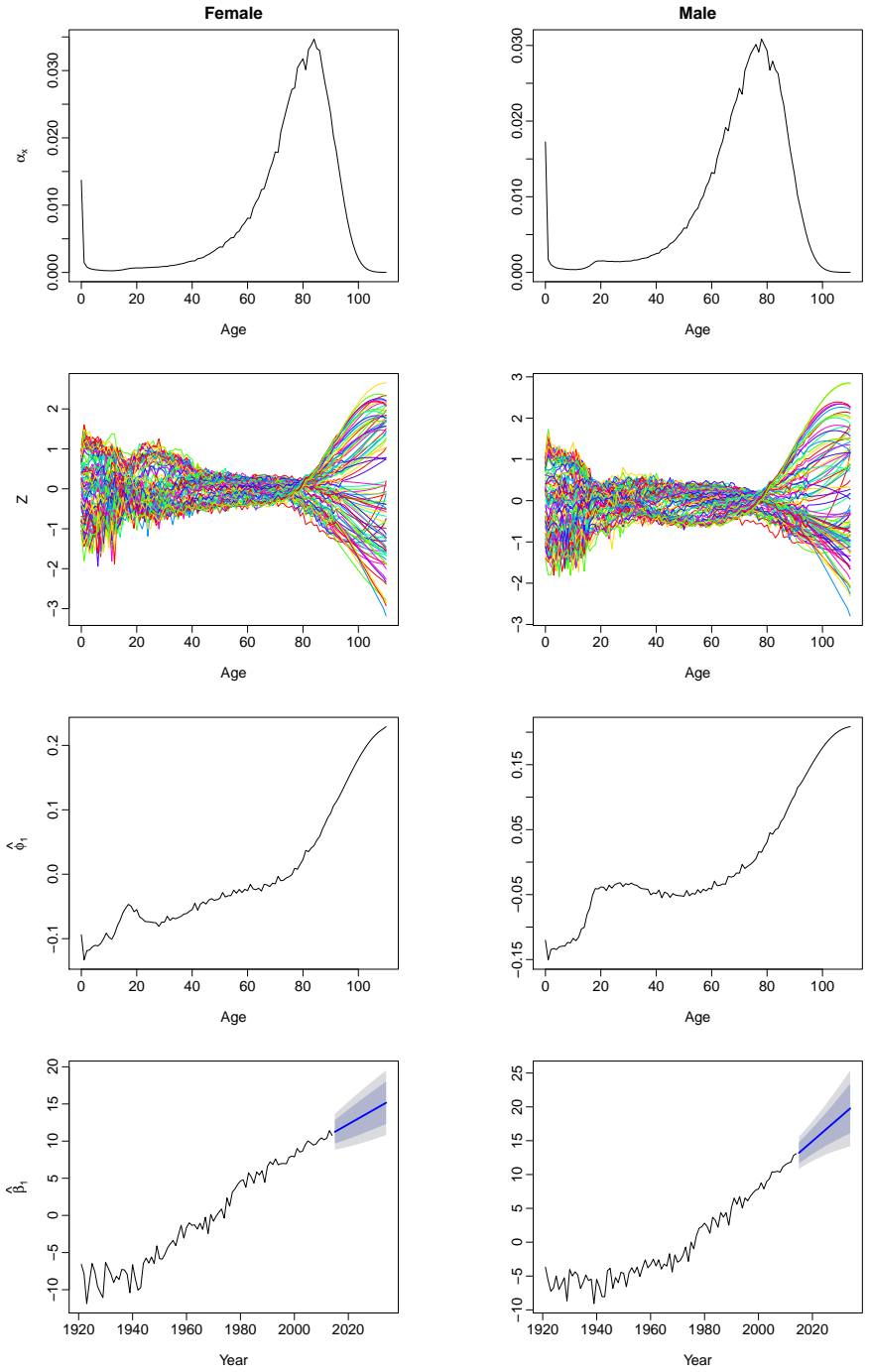
[Section 4 and Figure 2] The caption of Figure 2 says 'although we use L = 6 for fitting', while Section 4's R-squared discussion uses the CPV-selected L=1 and L=2; please clarify which value of L is used in the figure and in the goodness-of-fit calculations.
[Section 4] The text states that 'using the CPV criterion, we select L = 1 for both female and male data', but Section 3.1 reports L=1 for females and L=2 for males; this inconsistency should be resolved.

Circularity Check

1 steps flagged · score 6.0 of 10

CoDa's recommended L=6 is selected on the same holdout used to demonstrate its superiority, making the headline comparison partially circular.

fitted input called prediction [Sections 3.1, 4, 5.1-5.2, and 7]
"To determine the number of components L in (2) and (3), we consider a criterion known as cumulative percentage of variance (CPV) ... For the Australian female and male data, the chosen number of components L = 1 and L = 2, respectively. ... As a sensitivity analysis, we also consider setting the number of components to be L = 6 (see also Hyndman and Booth 2008). ... setting L = 6, including additional principal component decomposition pairs, generally provides more accurate point and interval forecast accuracies than setting L = 1 or L = 2 for the Australian female and male data."

The CPV rule is the paper's stated L-selection criterion and gives L=1 for females and L=2 for males. L=6 is introduced only as a sensitivity analysis and is adopted as the recommended configuration because the same holdout results in Table 1 show better MAPE and interval scores. Those holdout results are produced by the expanding-window procedure in Section 5.1, which is then used as the evidence for the paper's conclusion that 'the CoDa method with the ETS forecasting method and L = 6 is recommended, as it outperforms' the benchmarks. Thus the headline claim is not an independent out-of-sample evaluation of a pre-specified model: the model was selected by inspecting the very holdout outcomes that are later reported as evidence.

full rationale

No equation-level circularity exists in the CoDa forecasting algebra itself: the paper extrapolates principal-component scores with ETS and compares those forecasts against holdout death counts, rather than against fitted values. However, the central empirical claim of CoDa superiority is partially circular because the recommended L=6 is not selected by the stated CPV rule; it is chosen because it performed best on the same expanding-window holdout that is subsequently used to claim out-of-sample superiority. The conclusion that CoDa-ETS with L=6 outperforms HU, LC, and random walks therefore reduces, for the recommended configuration, to 'the configuration that scored best on the holdout scored best on the holdout.' The paper's acknowledged q=1-exp(-m) approximation in converting LC/HU mortality-rate forecasts to death counts is a benchmark-implementation fairness concern, not a circularity. Self-citations to prior work by the authors and collaborators are present but are not load-bearing for the forecast comparison; the core comparison is an empirical evaluation rather than a derivation from cited theorems. Because the headline forecast-accuracy claim is partly manufactured by test-set model selection, the circularity score is 6 rather than lower.

Assumptions & free parameters 4 free parameters · 6 assumptions · 0 invented entities

The central claim rests on a handful of domain assumptions common to functional mortality forecasting, plus two data-driven hyperparameters and an actuarial discount rate assumption. No new entities are introduced.

free parameters (4)

Number of retained principal components L = L=1 or 2 under CPV=85%; L=6 in sensitivity analysis
Selecting L is data-driven and affects all forecasts; L=6 is recommended because it lowers holdout errors, a choice made on the evaluation data.
Cumulative percentage of variance threshold delta = 0.85
Conventional threshold from Horvath and Kokoszka (2012, p.41) used to choose L; another threshold would change L and the forecasts.
Interest rate eta for annuity discounting = 3% per annum
Annuity prices are computed with B(0,tau)=exp(-eta*tau); the pricing results depend on this actuarial assumption.
Bootstrap replication count B = 1000
Number of bootstrap samples for prediction intervals; chosen by the authors and affects the precision of interval estimates, not the point forecasts.

assumptions (6)

domain assumption Life-table death counts are compositional data; the centered log-ratio transformation removes the unit-sum constraint without loss of information.
Underpins the entire CoDa framework in Section 3.1; standard in Aitchison (1986) but is a modeling choice.
domain assumption The transformed death counts follow a low-dimensional principal component structure, so the first L components capture the temporal dynamics.
Used in equation (2) and in forecasting step (3); if the dominant components shift over time, the forecast will be misspecified.
domain assumption Principal component scores can be extrapolated with univariate time series models, with ETS selected by AICc.
Used in Step 5 of Section 3.1; assumes the scores have forecastable temporal dependence.
domain assumption The approximation q = 1 - exp(-m) adequately converts central mortality rate forecasts to death-count forecasts for LC and HU.
Section 3.3.1; the paper concedes this conversion may explain the poorer LC/HU results.
domain assumption Residuals and h-step-ahead score forecast errors are exchangeable, so resampling them with replacement yields valid prediction intervals.
Required for the proposed bootstrap in Section 3.2.1; no coverage check is reported.
domain assumption Period life-table death count forecasts can be used to construct cohort survival probabilities for annuity pricing.
Section 6 converts forecast death counts into tau p_x products and discounts them into annuity prices.

how reviews work

0 comments

Cite this review

Pith. "Pith review of Forecasting age distribution of death counts: An application to annuity pricing." pith.science (2026). https://pith.science/paper/TF7463D6

@misc{pith2026190801446,
  author       = {Pith},
  title        = {Pith review of: Forecasting age distribution of death counts: An application to annuity pricing},
  year         = {2026},
  howpublished = {\url{https://pith.science/paper/TF7463D6}},
  note         = {Machine review of arXiv:1908.01446}
}

read the original abstract

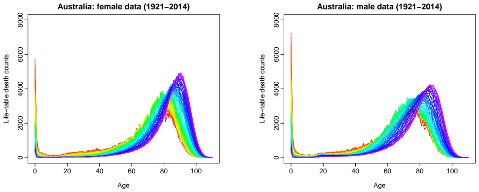
We consider a compositional data analysis approach to forecasting the age distribution of death counts. Using the age-specific period life-table death counts in Australia obtained from the Human Mortality Database, the compositional data analysis approach produces more accurate one- to 20-step-ahead point and interval forecasts than Lee-Carter method, Hyndman-Ullah method, and two na\"{i}ve random walk methods. The improved forecast accuracy of period life-table death counts is of great interest to demographers for estimating survival probabilities and life expectancy, and to actuaries for determining temporary annuity prices for various ages and maturities. Although we focus on temporary annuity prices, we consider long-term contracts which make the annuity almost lifetime, in particular when the age at entry is sufficiently high.

Figures

Figures reproduced from arXiv: 1908.01446 by the authors.

**Figure 1.** Rainbow plots of age-specific life-table death count from 1921 to 2014 in a single-year group. The oldest years are shown in red, with the most recent years in violet. Curves are ordered chronologically according to the colours of the rainbow. where the peaks shift to higher ages for both females and males. This shift is a primary source of the longevity risk, which is a major issue for insurers and pension funds, e… view at source ↗

**Figure 2.** Elements of the CoDa method for analysing the female and male age-specific life-table death counts in Australia. We present the first principal component and its scores, although we use L = 6 for fitting [PITH_FULL_IMAGE:figures/full_fig_p014_2.png] view at source ↗

**Figure 3.** A comparison of the point and interval forecast accuracy, as measured by the MAPE and mean interval score, among the CoDa, HU, LC and two na¨ıve RW methods using the holdout sample of the Australian female and male data. In the CoDa method, we use the ETS forecasting method with the number of principal components L = 6 [PITH_FULL_IMAGE:figures/full_fig_p019_3.png] view at source ↗

Figures from the paper (1 more)

**Figure 4.** Figure 4: Age-specific life-table death count forecasts from 2015 to 2064 for Australian females. The price of an annuity with a maturity term of a T year is a random variable, as it depends on the value of zero-coupon bond price and future mortality. The annuity price can be wr…

Discussion (0). Continue with ORCID to comment.

Reference graph

Works this paper leans on

4 extracted references · 4 canonical work pages

[1]

Aburto, J. M. and van Raalte, A. A. (2018), ‘LifeLife dispersion in times of life expectancy ﬂuctuation: The case of central and eastern Europe’, Demography 55, 2071–2096. Aitchison, J. (1982), ‘The statistical analysis of compositional data’,Journal of the Royal Statistical Society: Series B 44(2), 139–177. Aitchison, J. (1986), The Statistical Analysis ...

work page 2018
[4]

If age + maturity > 110, NA will be shown in the table. Age T = 5 T = 10 T = 15 T = 20 T = 25 T = 30 CPV 60 4.4821 8.1694 11.1358 13.4387 15.0911 16.1213 65 4.4417 8.0150 10.7890 12.7794 14.0204 14.5930 70 4.3779 7.7766 10.2151 11.7356 12.4372 12.6353 75 4.2734 7.3396 9.2514 10.1336 10.3827 10.4173 80 4.0425 6.5631 7.7262 8.0546 8.1001 8.1027 85 3.6839 5....

work page
[110]

These estimates are based on forecast mortality rates from 2015 to

Table 4: Estimates of annuity prices with different ages and maturities ( T) for a male policyholder residing in Australia. These estimates are based on forecast mortality rates from 2015 to

work page 2015
[2017]

Forecasting age distribution of death counts: An application to annuity pricing

URL: http://www. mortality.org. Hurvich, C. M. and Tsai, C.-L. (1993), ‘A corrected Akaike information criterion for vector autoregressive model selection’,Journal of Time Series Analysis 14(3), 271–279. Hyndman, R. J., Athanasopoulos, G., Bergmeir, C., Caceres, G., Chhay, L., O’Hara-Wild, M., Petropoulos, F., Razbash, S., Wang, E., Yasmeen, F., Team, R. ...

work page 1993

Pith tools

Reviewed August 14, 2026 · model on record in the stance chip above.

[1] [1]

Aburto, J. M. and van Raalte, A. A. (2018), ‘LifeLife dispersion in times of life expectancy ﬂuctuation: The case of central and eastern Europe’, Demography 55, 2071–2096. Aitchison, J. (1982), ‘The statistical analysis of compositional data’,Journal of the Royal Statistical Society: Series B 44(2), 139–177. Aitchison, J. (1986), The Statistical Analysis ...

work page 2018

[2] [4]

If age + maturity > 110, NA will be shown in the table. Age T = 5 T = 10 T = 15 T = 20 T = 25 T = 30 CPV 60 4.4821 8.1694 11.1358 13.4387 15.0911 16.1213 65 4.4417 8.0150 10.7890 12.7794 14.0204 14.5930 70 4.3779 7.7766 10.2151 11.7356 12.4372 12.6353 75 4.2734 7.3396 9.2514 10.1336 10.3827 10.4173 80 4.0425 6.5631 7.7262 8.0546 8.1001 8.1027 85 3.6839 5....

work page

[3] [110]

These estimates are based on forecast mortality rates from 2015 to

Table 4: Estimates of annuity prices with different ages and maturities ( T) for a male policyholder residing in Australia. These estimates are based on forecast mortality rates from 2015 to

work page 2015

[4] [2017]

Forecasting age distribution of death counts: An application to annuity pricing

URL: http://www. mortality.org. Hurvich, C. M. and Tsai, C.-L. (1993), ‘A corrected Akaike information criterion for vector autoregressive model selection’,Journal of Time Series Analysis 14(3), 271–279. Hyndman, R. J., Athanasopoulos, G., Bergmeir, C., Caceres, G., Chhay, L., O’Hara-Wild, M., Petropoulos, F., Razbash, S., Wang, E., Yasmeen, F., Team, R. ...

work page 1993