REVIEW 5 minor 36 references
Fair Box ordinate transform for forecasts following a multivariate Gaussian law
T0 review · 0 major / 5 minor · reviewed 2026-08-06 · deepseek-v4-flash
Pith's one-line read The paper derives a fair sample Box ordinate transform that is exactly uniform for any ensemble size when forecasts are calibrated multivariate Gaussians, and shows it detects miscalibration where earlier sample versions fail.
desk verdict A clean, correctly-derived exact small-sample BOT for Gaussian ensemble forecasts; modest but genuinely useful, and honestly reported. read the letter →
The pith
A machine-rendered reading of the paper's core claim, the machinery that carries it, and where it could break.
The reading
What carries the argument
The load-bearing object is the exact sampling distribution of the Mahalanobis distance between a new Gaussian observation and the sample mean of an iid Gaussian ensemble, using the sample covariance matrix. Because the sample mean $m$ and the sample covariance $S$ are independent, $m\sim N_p(\mu, n^{-1}\Sigma)$ and $(n-1)S$ follows a Wishart law, the rescaled statistic $Y=\sqrt{n/(n+1)}(x_0-m)$ is $N_p(0,\Sigma)$ and independent of $S$, so the squared distance $T^2=\frac{n}{n+1}(x_0-m)^\top S^{-1}(x_0-m)$ follows Hotelling's $T^2$ distribution with $p$ and $n-1$ degrees of freedom. The proportionality $T^2 \propto F_{p,n-p}$ then supplies the closed-form CDF used in Eq. (2.5). The device that makes the transform 'fair' is replacing the asymptotic chi-square CDF of the classical BOT with this exact $F$ CDF, evaluated at the ensemble-size- and dimension-dependent scale $\frac{n(n-p)}{p(n^2-1)}$ of the observed squared distance; this single substitution is what makes the null distribution exactly uniform for all $n>p$ and what keeps the diagnostic's power aligned with the theoretical BOT.
What would settle it
Run $10^5$ replicates with $x_0,x_1,\ldots,x_n$ drawn independently from $N_p(0,I_p)$ for $n=p+1$ and $p\in\{2,5,10\}$, compute the fair BOT values, and count Kolmogorov-Smirnov rejections at the 5% level; the rejection rate must stay at 5% for the exact-uniformity claim to stand. A companion run with exchangeable but dependent members — for instance, all members sharing a common latent shift with the verifying observation — would settle whether the guarantee extends to the 'exchangeable ensemble' language used in the operational part of the paper, which the derivation itself does not cover.
Extended reading notes
Core claim
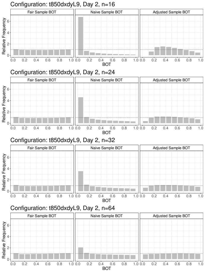
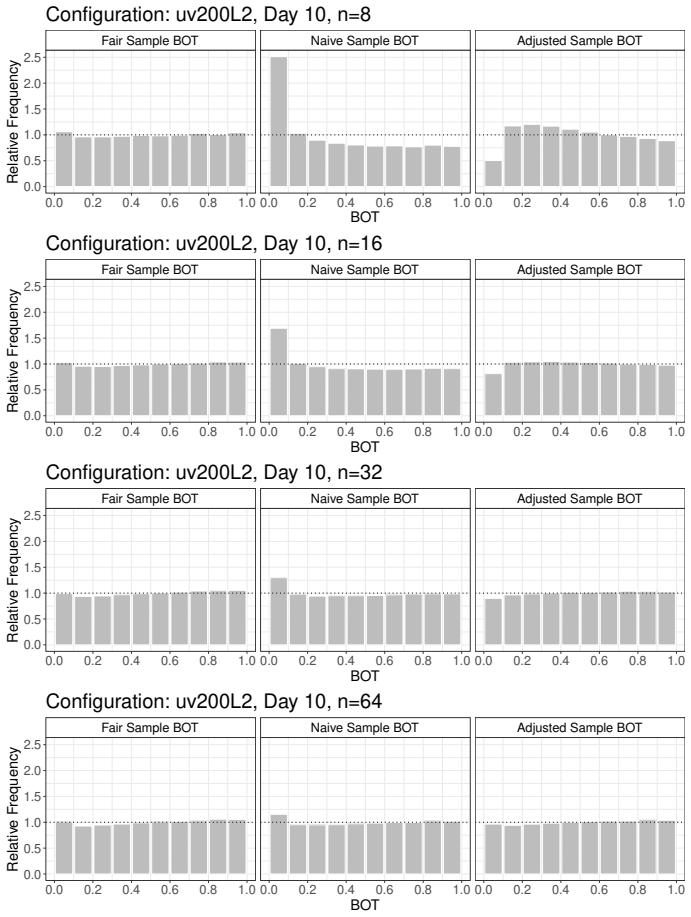
The paper claims that when a $p$-dimensional forecast is represented by an $n$-member ensemble that, together with the verifying observation, forms an independent sample from one common Gaussian law, the fair sample BOT $$u^F_n(m,S;x_0) = 1 - F_{p,n-p}\!\left[\frac{n(n-p)}{p($n^{2}$-1)}(x_0-m)^\top $S^{{-1}}$(x_0-m)\right]$$ is exactly standard uniform for every $n>p$. The reason is that the rescaled squared Mahalanobis distance $\frac{n}{n+1}(x_0-m)^\top S^{-1}(x_0-m)$ follows Hotelling's $T^2$ distribution with $p$ and $n-1$ degrees of freedom, and multiplying by $\frac{n-p}{p(n-1)}$ converts it to an $F_{p,n-p}$ variable whose CDF is known in closed form. This removes the asymptotic 'large $n$' assumption carried by the naive sample BOT and by the adjusted version that includes the observation in the parameter estimates. In simulations, the fair BOT keeps Kolmogorov-Smirnov rejection rates at the nominal 5% for every tested combination of dimension and ensemble size, while the adjusted version needs hundreds to thousands of members before its test level approaches 5%. The paper also shows the fair BOT mimics the theoretical BOT histogram shapes under variance, correlation, and mean miscalibration, and it states explicitly that a flat fair BOT histogram is necessary but not sufficient for reliability, because compensating variance and correlation errors across coordinates can cancel inside the quadratic form.
Load-bearing premise
The entire construction assumes the $n$ ensemble members and the verifying observation are independent draws from one common multivariate Gaussian distribution; if members are mutually dependent, merely exchangeable, or the forecast law is not Gaussian, exact uniformity is lost.
Editorial extensions
If this is right
- Calibration of Gaussian ensemble forecasts can be assessed as soon as the ensemble has more members than the forecast has dimensions, dropping the $n\gg p$ requirement (about 100 members for $p=3$) that earlier sample BOTs needed.
- Because calibrated forecasts give exactly uniform fair BOT values, a Kolmogorov-Smirnov test on the values is a valid formal test of calibration at any ensemble size, rather than only an asymptotic approximation.
- Under misspecified covariance or bias in the mean, the fair BOT histograms keep the same shapes as the theoretical BOT histograms, so miscalibration is detectable at ensemble sizes where the naive and adjusted versions are badly biased or useless.
- A flat fair BOT histogram is not proof of reliability: alternating-sign variance or correlation errors across coordinates can compensate inside the quadratic form, so the authors recommend combining the fair BOT with marginal rank histograms and lower-dimensional fair BOTs.
- On operationally verified weather data, the fair BOT shows nearly flat histograms for near-Gaussian, nearly calibrated configurations and reveals bias in temperature stencils and wind profiles, with $\cup$-shaped departures when the data fail multivariate normality tests.
Reading between the lines
- The Hotelling-to-$F$ rescaling is generic: any quadratic-form diagnostic computed from a Gaussian sample mean and covariance — for example checks restricted to fixed lower-dimensional subspaces of a forecast vector — could be made exactly independent of ensemble size by the same device, with no new distribution theory.
- A testable extension: apply the fair BOT to forecasts first transformed toward Gaussianity (Box-Cox marginals or copula-based post-processing, approaches the authors mention), and check whether the $\cup$-shapes seen in raw non-Gaussian configurations flatten; that would separate the normality assumption from genuine miscalibration as the source of the departure.
- For operational use, the derivation's independence requirement is stronger than the exchangeability that real ensembles satisfy; a dedicated simulation with exchangeable-but-dependent members would quantify how much the uniform guarantee degrades under realistic member dependence.
Editorial analysis
A structured set of objections, weighed in public.
Referee Report
Summary. The paper introduces a "fair" version of the Gaussian sample Box ordinate transform (BOT) for assessing calibration of multivariate ensemble forecasts. Section 2 derives Eq. (2.5), which transforms the squared Mahalanobis distance between the observation and the ensemble mean, scaled by the ensemble covariance, using an F_{p,n-p} cumulative distribution function. Under the stated assumption that the observation and the n ensemble members are independent and identically distributed draws from a common p-dimensional Gaussian distribution, the transform is shown to be exactly standard uniform for any ensemble size n > p. The simulation study in Section 3 compares the fair BOT with the theoretical, naive, and adjusted sample BOTs across several dimensions, ensemble sizes, and miscalibration types (variance, correlation, and mean bias). Section 4 presents applications to operational ECMWF ensemble forecasts in four multivariate configurations, both in a perfectly reliable setting and in verification against analyses. The paper concludes that the fair BOT provides flat histograms for calibrated Gaussian forecasts even for small ensemble sizes, and that it qualitatively reproduces the shapes of the theoretical BOT under miscalibration, while also acknowledging that flat histograms do not guarantee reliability because of possible compensating errors.
Significance. The contribution is useful and timely: it provides an exact, parameter-free calibration diagnostic for multivariate Gaussian ensemble forecasts that remains valid for small ensemble sizes, which is a practical gap in the existing BOT methodology. The central derivation in Section 2 is a textbook application of Hotelling's T^2 theory, and the resulting transform is simple to implement. The simulation study is extensive and includes power curves for detecting covariance miscalibration, and the ECMWF examples give a realistic testbed. The paper is honest about its main limitation—the Gaussian and independence assumptions—and explicitly recommends supplementary checks such as univariate rank histograms and lower-dimensional fair BOTs. The results, if accepted, should be of interest to researchers and practitioners in forecast verification.
minor comments (5)
- [Appendix B.3] The heading and opening sentence of Appendix B.3 refer to the "10-dimensional predictand" of vector wind, but the configuration uv200to925L12 is 12-dimensional (six levels of horizontal vector wind), as correctly stated in Section 4.2.3; please correct this inconsistency.
- [Section 4.2.2] In the description of the adjusted sample BOT histograms near the end of Section 4.2.2, the word "asymetric" should be "asymmetric".
- [Section 2] The opening sentence "Assume, that the predictive distribution..." contains an unnecessary comma; it should read "Assume that the predictive distribution...".
- [Section 3.2.1] The phrase "misscalibration" appears in the first sentence of Section 3.2.1; this should be "miscalibration".
- [Figure 4 caption] The caption of Figure 4 contains a line break inside "simulatio ns"; please fix the typesetting so the word "simulations" is not split incorrectly.
Circularity Check
No significant circularity; the fair BOT is derived from classical Hotelling T-squared distribution theory.
full rationale
The derivation of the fair Gaussian sample BOT is self-contained and not circular. Section 2 derives Eq. (2.4) from textbook distribution theory (H?rdle and Simar 2019, Theorems 5.7 and 5.9): for iid Gaussian ensemble members and observation, the sample mean and covariance are independent, the rescaled difference Y is N_p(0,Sigma), and the scaled squared Mahalanobis distance follows Hotelling's T^2_{p,n-1}, hence F_{p,n-p}. Eq. (2.5) is then the probability integral transform of that known distribution, so uniformity under the calibrated-Gaussian assumption is a theorem, not a fitted parameter or an assumed ansatz. No constant is tuned to make the histograms flat; the n- and p-dependent scaling is derived, not optimized. The simulations are a check of the theorem under the stated assumptions, and the ECMWF application is empirical. The authors' self-citations (Leutbecher and Baran 2025) are used for the HZ normality assessment of the ECMWF configurations and as motivation, but they are not load-bearing for the mathematical derivation. The paper itself flags limitations in Section 5 ('valid for forecasts following a multivariate Gaussian law') and in Section 3.2.1 (flat histograms despite compensating miscalibration); these are validity caveats, not circularity. Similarly, the operational members are exchangeable rather than independent, so the exact-uniformity theorem does not formally cover those experiments, but the paper does not claim the theorem for dependent members.
Assumptions & free parameters
assumptions (3)
- domain assumption Observation and ensemble members are iid draws from the same p-dimensional Gaussian distribution N_p(mu, Sigma)
- domain assumption The sample covariance matrix S is regular, requiring n > p
- standard math Classical distributional results: m and S are independent, (n-1)S ~ W_p(n-1, Sigma), and the Hotelling T-squared to F transformation
Cite this review
Pith. "Pith review of Fair Box ordinate transform for forecasts following a multivariate Gaussian law." pith.science (2026). https://pith.science/paper/TIGN4XOO
@misc{pith2026250622601,
  author       = {Pith},
  title        = {Pith review of: Fair Box ordinate transform for forecasts following a multivariate Gaussian law},
  year         = {2026},
  howpublished = {\url{https://pith.science/paper/TIGN4XOO}},
  note         = {Machine review of arXiv:2506.22601}
}
abstract
Monte Carlo techniques are the method of choice for making probabilistic predictions of an outcome in several disciplines. Usually, the aim is to generate calibrated predictions which are statistically indistinguishable from the outcome. Developers and users of such Monte Carlo predictions are interested in evaluating the degree of calibration of the forecasts. Here, we consider predictions of $p$-dimensional outcomes sampling a multivariate Gaussian distribution and apply the Box ordinate transform (BOT) to assess calibration. However, this approach is known to fail to reliably indicate calibration when the sample size n is moderate. For some applications, the cost of obtaining Monte-Carlo estimates is significant, which can limit the sample size, for instance, in model development when the model is improved iteratively. Thus, it would be beneficial to be able to reliably assess calibration even if the sample size n is moderate. To address this need, we introduce a fair, sample size- and dimension-dependent version of the Gaussian sample BOT. In a simulation study, the fair Gaussian sample BOT is compared with alternative BOT versions for different miscalibrations and for different sample sizes. Results confirm that the fair Gaussian sample BOT is capable of correctly identifying miscalibration when the sample size is moderate in contrast to the alternative BOT versions. Subsequently, the fair Gaussian sample BOT is applied to two to 12-dimensional predictions of temperature and vector wind using operational ensemble forecasts of the European Centre for Medium-Range Weather Forecasts (ECMWF). Firstly, perfectly reliable situations are considered where the outcome is replaced by a forecast that samples the same distribution as the members in the ensemble. Secondly, the BOT is computed using estimates of the actual temperature and vector wind from ECMWF analyses.
Figures


Figures from the paper (21 more)






Reference graph
Works this paper leans on
-
[1]
Allen, S., Ziegel, J. and Ginsbourger, D. (2024) Assessing the calibration of multivariate probabilistic forecasts. Quarterly Journal of the Royal Meteorological Society, 150, 1315--1335
work page 2024
-
[2]
Baran, S., Hemri, S. and El Ayari, M. (2019) Statistical postprocessing of water level forecasts using bayesian model averaging with doubly truncated normal components. Water Resources Research, 55, 3997--4013
work page 2019
-
[3]
(2025) Casting light on dependency structures in ensemble forecasts with the 2-d rank histogram
Ben Bouall \`e gue, Z. (2025) Casting light on dependency structures in ensemble forecasts with the 2-d rank histogram. Meteorological Applications, 32, e70057
work page 2025
-
[4]
Berrocal, V. J., Raftery, A. E., Gneiting, T. and Steed, R. C. (2010) Probabilistic weather forecasting for winter road maintenance. Journal of the American Statistical Association, 105, 522--537
work page 2010
-
[5]
25 years of ensemble forecasting
Buizza, R. (2018a) Introduction to the special issue on “25 years of ensemble forecasting”. Quarterly Journal of the Royal Meteorological Society, 145, 1--11
work page 2018
-
[6]
In Statistical Postprocessing of Ensemble Forecasts (eds
--- (2018b) Ensemble forecasting and the need for calibration. In Statistical Postprocessing of Ensemble Forecasts (eds. S. Vannitsem, D. S. Wilks and J. W. Messner), 15--48. Amsterdam: Elsevier
work page 2018
-
[7]
Chen, J., Janke, T., Steinke, F. and Lerch, S. (2024) Generative machine learning methods for multivariate ensemble postprocessing. The Annals of Applied Statistics, 18, 159--189
work page 2024
-
[8]
Dai, Y. and Hemri, S. (2021) Spatially coherent postprocessing of cloud cover ensemble forecasts. Monthly Weather Review, 49, 3923--3937
work page 2021
Show all 36 references
-
[9]
J., Kneringer, P., Mayr, G
Dietz, S. J., Kneringer, P., Mayr, G. J. and Zeileis, A. (2019) Low-visibility forecasts for different flight planning horizons using tree-based boosting models. Advances in Statistical Climatology, Meteorology and Oceanography, 5, 101--114
2019
-
[10]
K., Gao, X
Duan, Q., Ajami, N. K., Gao, X. and Sorooshian, S. (2007) Multi-model ensemble hydrologic prediction using bayesian model averaging. Advances in Water Resources, 30, 1371--1386
2007
-
[11]
Reading: ECMWF
ECMWF (2024) IFS Documentation CY49R1 -- Part V: Ensemble Prediction System. Reading: ECMWF
2024
-
[12]
Ferro, C. A. T. (2014) Fair scores for ensemble forecasts. Quarterly Journal of the Royal Meteorological Society, 140, 1917--1923
2014
-
[13]
Ferro, C. A. T., Richardson, D. S. and Weigel, A. P. (2008) On the effect of ensemble size on the discrete and continuous ranked probability scores. Meteorological Applications, 15, 19--24
2008
-
[14]
E., Ferro, C
Fricker, T. E., Ferro, C. A. T. and Stephenson, D. B. (2013) Three recommendations for evaluating climate predictions. Meteorological Applications, 20, 246--255
2013
-
[15]
and Raftery, A
Gneiting, T. and Raftery, A. E. (2007) Strictly proper scoring rules, prediction and estimation. Journal of the American Statistical Association, 102, 359--378
2007
-
[16]
I., Grimit, E
Gneiting, T., Stanberry, L. I., Grimit, E. P., Held, L. and Johnson, N. A. (2008) Assessing probabilistic forecasts of multivariate quantities, with an application to ensemble predictions of surface winds. Test, 17, 211--235
2008
-
[17]
Good, I. J. (1952) Rational decisions. Journal of the Royal Statistical Society. Series B: Statistical Methodology, 14, 107--114
1952
-
[18]
Hamill, T. M. (2001) Interpretation of rank histograms for verifying ensemble forecasts. Monthly Weather Review, 129, 550--560
2001
-
[19]
H \"a rdle, W. K. and Simar, L. (2019) Applied Multivariate Statistical Analysis. Springer Nature, 5th edn
2019
-
[20]
and Zappa, M
Hemri, S., Fundel, F. and Zappa, M. (2013) Simultaneous calibration of ensemble river flow predictions over an entire range of lead times. Water Resources Research, 49, 6744--6755
2013
-
[21]
and Klein, B
Hemri, S., Lisniak, D. and Klein, B. (2015) Multivariate postprocessing techniques for probabilistic hydrological forecasting. Water Resources Research, 51, 7436--7451
2015
-
[22]
and Zirkler, B
Henze, N. and Zirkler, B. (1990) A class of invariant consistent tests for multivariate normality. Communications in Statistics -- Theory and Methods, 19, 3595--3617
1990
-
[23]
and Baran, S
Lakatos, M., Lerch, S., Hemri, S. and Baran, S. (2023) Comparison of multivariate post-processing methods using global ECMWF ensemble forecasts. Quarterly Journal of the Royal Meteorological Society, 149, 856--877
2023
-
[24]
Lang, S., Alexe, M., Clare, M. C. A., Roberts, C., Adewoyin, R., Bouallègue, Z. B., Chantry, M., Dramsch, J., Dueben, P. D., Hahner, S., Maciel, P., Prieto-Nemesio, A., O'Brien, C., Pinault, F., Polster, J., Raoult, B., Tietsche, S. and Leutbecher, M. (2024) Aifs-crps: Ensembl...
2024 arXiv
-
[25]
and Graeter, M
Lerch, S., Baran, S., M\"oller, A., Gro , J., Schefzik, R., Hemri, S. and Graeter, M. (2020) Simulation-based comparison of multivariate ensemble post-processing methods. Nonlinear Processes in Geophysics, 27, 349--371
2020
-
[26]
and Baran, S
Leutbecher, M. and Baran, S. (2025) Ensemble size dependence of the logarithmic score for forecasts issued as multivariate normal distributions. Quarterly Journal of the Royal Meteorological Society, 151, e4898
2025
-
[27]
and Palmer, T
Leutbecher, M. and Palmer, T. N. (2008) Ensemble forecasting. Journal of Computational Physics, 227, 3515--3539
2008
-
[28]
Lewis, J. M. (2005) Roots of ensemble forecasting. Monthly Weather Review, 133, 1865--1885
2005
-
[29]
R., El-Kadi, A., Masters, D., Ewalds, T., Stott, J., Mohamed, S., Battaglia, P., Lam, R
Price, I., Sanchez-Gonzalez, A., Alet, F., Andersson, T. R., El-Kadi, A., Masters, D., Ewalds, T., Stott, J., Mohamed, S., Battaglia, P., Lam, R. and Willson, M. (2025) Probabilistic weather forecasting with machine learning. Nature, 637, 84--90
2025
-
[30]
Richardson, C. W. (1981) Stochastic simulation of daily precipitation, temperature, and solar radiation. Water Resources Research, 17, 182--190
1981
-
[31]
(2016) Combining parametric low-dimensional ensemble postprocessing with reordering methods
Schefzik, R. (2016) Combining parametric low-dimensional ensemble postprocessing with reordering methods. Quarterly Journal of the Royal Meteorological Society, 142, 2463--2477
2016
-
[32]
Siegert, S., Ferro, C. A. T., Stephenson, D. . B. and Leutbecher, M. (2019) The ensemble-adjusted ignorance score for forecasts issued as normal\ distributions. Quarterly Journal of the Royal Meteorological Society, 145, 129--139
2019
-
[33]
L., Scheuerer, M
Thorarinsdottir, T. L., Scheuerer, M. and Heinz, C. (2016) Assessing the calibration of high-dimensional ensemble forecasts using rank histograms. Journal of Computational and Graphical Statistics, 25, 105--122
2016
-
[34]
B., Demaeyer, J., Evans, G
Vannitsem, S., Bremnes, J. B., Demaeyer, J., Evans, G. R., Flowerdew, J., Hemri, S., Lerch, S., Roberts, N., Theis, S., Atencia, A., Ben Bouall \`e gue , Z., Bhend, J., Dabernig, M., Cruz, L. D., Hieta, L., Mestre, O., Moret, L., Plenkovi \'c , I. O., Schmeits, M., Taillardat,...
2021
-
[35]
Wilks, D. S. (2017) On assessing calibration of multivariate ensemble forecasts. Quarterly Journal of the Royal Meteorological Society, 143, 164--172
2017
-
[36]
Amsterdam: Elsevier, 4th edn
--- (2019) Statistical Methods in the Atmospheric Sciences. Amsterdam: Elsevier, 4th edn
2019
Reviewed August 6, 2026 · model on record in the stance chip above.
Discussion (0). Continue with ORCID to comment.