REVIEW 4 major objections 5 minor 8 references
On the generalized method lines applied to the time-independent incompressible Navier-Stokes system
T0 review · 4 major / 5 minor · reviewed 2026-08-14 · deepseek-v4-flash
Pith's one-line read Solving a linear system yields exact steady Navier-Stokes solutions when the body force is a gradient.
desk verdict The exact theorem has a genuine topological gap (curl-free doesn't mean gradient on an annulus, and the pressure trace is overdetermined), and the numerical validation is a fit to the same residual it claims to confirm. read the letter →
The pith
A machine-rendered reading of the paper's core claim, the machinery that carries it, and where it could break.
The reading
What carries the argument
The central object is the three-potential velocity ansatz $u=\partial_x w_0+\partial_x w_1+\partial_y w_2$, $v=\partial_y w_0-\partial_y w_1-\partial_x w_2$. The two equations in (8) serve two purposes: $\nabla^2 w_0+\partial_{xx}w_1-\partial_{yy}w_1=0$ enforces incompressibility, and $\nabla^2 w_2+2\partial_{xy}w_1=0$ makes the vorticity of $(u,v)$ vanish. Together they make the nonlinear convective terms curl-free, so the momentum equations reduce to a gradient and can be integrated to a pressure. The generalized method of lines discretizes one coordinate, here the radial variable, into a set of lines, writes the solution on each line as a function of the boundary data and the line index, and solves the resulting coupled system by a Banach fixed-point iteration.
What would settle it
Solve (8) with boundary data $u_0=-y$, $v_0=x$ on the outer circle and no-slip on the inner circle. Any field produced by (7) has zero vorticity, while the prescribed outer trace has non-zero circulation, so either the linear system has no solution or the resulting velocity fails the momentum equation; this would settle whether Theorem 2.1 holds for arbitrary boundary data.
Extended reading notes
Core claim
Theorem 2.1 claims that for a gradient body force $(\partial_x f,\partial_y f)$, the velocity field defined by $u=\partial_x w_0+\partial_x w_1+\partial_y w_2$ and $v=\partial_y w_0-\partial_y w_1-\partial_x w_2$ solves the steady incompressible Navier-Stokes system whenever $w_0,w_1,w_2$ satisfy the linear system $\nabla^2 w_2+2\partial_{xy}w_1=0$, $\nabla^2 w_0+\partial_{xx}w_1-\partial_{yy}w_1=0$, together with the boundary conditions on $u$ and $v$. The pressure $P$ is then obtained by integrating the curl-free momentum equations with $P=P_0$ on the outer boundary. The load-bearing identity is (9): when the two auxiliary equations hold, the curl of the convective terms vanishes, so the momentum operator is curl-free and a scalar pressure exists. A direct consequence is that the resulting flow has zero vorticity. The paper's second part extends this to approximate solutions, actually for the regularized system (25) with a small parameter $\varepsilon$, by the generalized method of lines, using a Banach fixed-point iteration on each line and minimizing the $L^2$ residual (29).
Load-bearing premise
The boundary data must be traces of a curl-free velocity field with a single-valued pressure around the hole; the paper states the boundary conditions without verifying this compatibility.
Editorial extensions
If this is right
- If Theorem 2.1 is correct, an exact steady incompressible Navier-Stokes solution follows from solving the linear system (8) for any gradient body force, without iterating on the nonlinear terms.
- The method-of-lines formulas, with coefficients obtained by minimizing the residual $J$, give explicit approximate velocity and pressure fields on each line that can serve as initial guesses or manufactured solutions for Navier-Stokes computations.
- Because the exact constructed flows are irrotational, they form a potential-flow subclass of the steady Navier-Stokes solutions; their pressure is recovered from a gradient, so the boundary pressure datum determines the integration constant.
- The paper announces the extension to three-dimensional, compressible, and time-dependent cases as future work.
Reading between the lines
- The theorem's exact solutions are necessarily potential flows: the first equation of (8) forces zero vorticity, so the boundary data admitted by the construction are only those compatible with an irrotational velocity field, even though the theorem states the boundary conditions without this restriction.
- On a doubly connected domain, recovering a single-valued pressure from a curl-free momentum equation requires a compatibility condition around the inner boundary; checking whether the pressure returns to its starting value after one loop would provide a direct test of the construction.
- The same three-potential trick could turn other conservative-force fluid models, such as steady magnetohydrodynamics with a gradient magnetic-pressure term, into linear problems if the additional force can be written as a gradient.
Signed reviews
Editorial analysis
A structured set of objections, weighed in public.
Referee Report
Summary. The manuscript has two parts. In the first part, Theorem 2.1 claims that for a gradient body force h=(∂x f, ∂y f), any solution of the linear system (8) for potentials w0, w1, w2 yields an exact solution of the steady incompressible Navier-Stokes system with boundary conditions (6), including a prescribed pressure P=P0 on the outer boundary Γ1. The proof shows that the momentum residual is curl-free and asserts that a pressure can then be recovered. In the second part, the paper proposes a semi-discrete 'generalized method of lines' for an approximate system (25), states that the iteration is solved through the Banach fixed point theorem, presents explicit line formulas for u, v, and P, and reports two numerical examples in which coefficients are obtained by minimizing the residual functional J in (29).
Significance. If Theorem 2.1 were correct, it would be a surprising exact reduction of a nonlinear PDE system to a linear one for gradient forces, and the explicit line formulas could be of practical interest. The algebraic identity in equations (9)-(11) is checkable, and the manuscript is transparent that the numerical coefficients come from minimizing J. However, the central theorem is not proven as stated: the pressure recovery on an annulus is unjustified, the constructed velocity is forced to be irrotational without stating compatibility conditions on the boundary data, and no existence proof is given for the potentials. The numerical evidence is also circular because the same minimized functional J is quoted as evidence of accuracy. The paper does not supply machine-checkable proofs, reproducible code, or a falsifiable prediction that would compensate for these gaps.
major comments (4)
- [Theorem 2.1, proof after Eq. (11)] Equation (11) establishes only that the momentum residual F is curl-free. On the doubly connected domain Ω, a curl-free field need not be a gradient: one must also verify zero circulation around the inner boundary Γ0. Even if F = ∇P, the potential P is determined only up to an additive constant, so the additional condition P = P0 on the whole of Γ1 is not automatically satisfiable; it requires a compatibility condition. The sentence 'we may obtain P which satisfies the concerning boundary condition' after (12) is unsupported, so the central claim that solving (8) yields a solution of (5)-(6) is not established.
- [Theorem 2.1, Eqs. (7)-(8)] The constraint ∇²w2 + 2∂xyw1 = 0 forces the constructed velocity to be irrotational, since ∂xv − ∂yu = −(∇²w2 + 2∂xyw1) = 0. The boundary data u0, v0 in (6) are therefore not arbitrary; they must be compatible with an irrotational, divergence-free extension, and the theorem states no such compatibility condition. Moreover, the proof begins by assuming w0, w1, w2 exist and never gives an existence argument for the system (8) with general boundary data, so the theorem is incomplete even as a conditional statement.
- [Section 3, fixed-point iteration after Eq. (24)] The paper states that the equations are solved through the Banach fixed point theorem, but it does not specify the complete metric space, the norm, or the contraction estimate for the maps T̂n. The displayed iteration is merely a Picard iteration; without a contraction proof it does not establish convergence. This gap affects the method-of-lines existence claim advertised in the abstract and the conclusion.
- [Section 3.1, Eq. (29)] The coefficients {ai[n]}, {bi[n]}, {ci[n]} are obtained by minimizing J, and the same minimized J is then reported as evidence that the approximations are good ('it seems we have got good first approximations'). This is circular: a small J only shows that the ansatz (26)-(28) can fit the two chosen examples, not that the generalized method of lines predicts the Navier-Stokes solution. The general line expressions are not derived from the fixed-point scheme; they are fitting templates whose parameters are chosen to minimize the residual.
minor comments (5)
- [Theorem 2.1, statement] The phrase 'P is a solution of the system indicated in the first two lines of (25)' is confusing because (25) is introduced later and contains the regularization parameter ε; the theorem should state the momentum equations explicitly.
- [Eq. (23) and line formulas] There are subscript and notation typos, such as 'd̂1(v,vn−1)' in (23), which appears to be 'd̂1(vn, vn−1)', and similar omissions in the displayed line formulas.
- [Section 3.1, boundary conditions] The text says that in the numerical examples there are no boundary conditions for the pressure, but it also states that P0 must be calculated numerically in the optimization process; the role of P0 in (26)-(28) needs clarification.
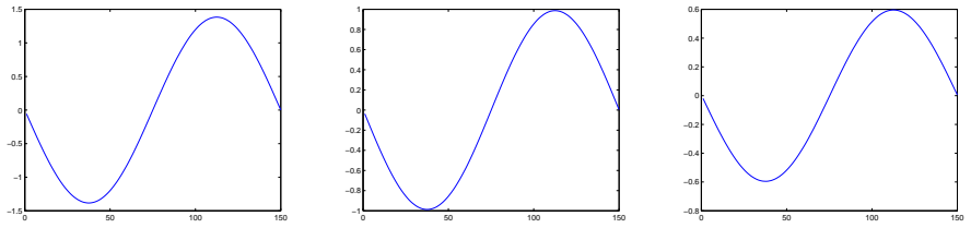
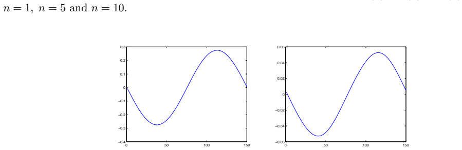
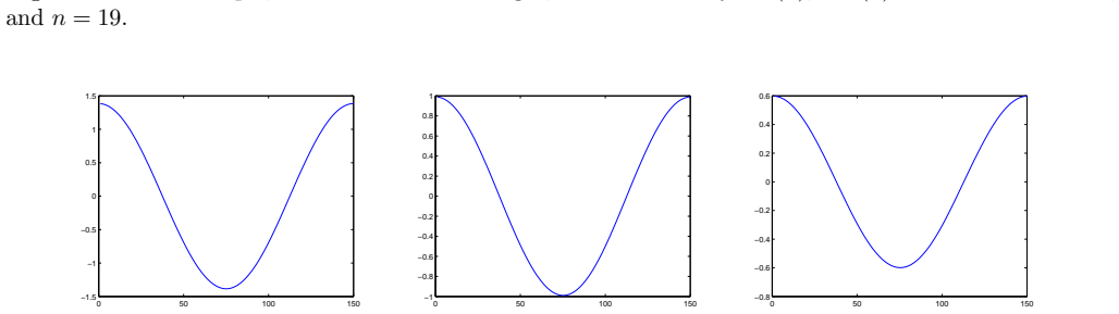
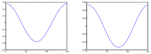
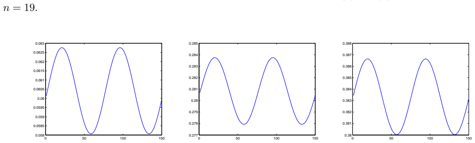
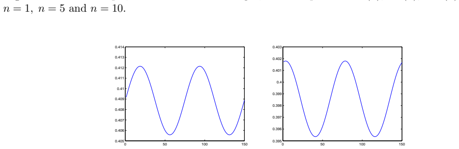
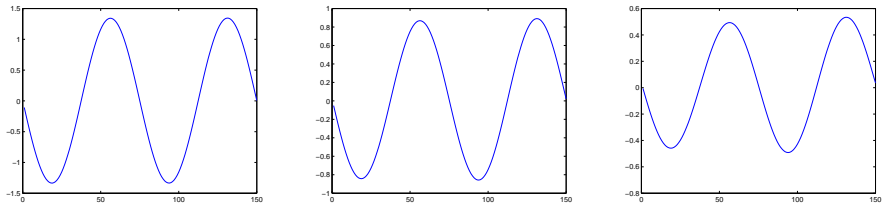
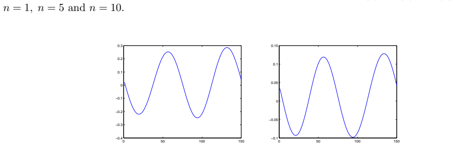
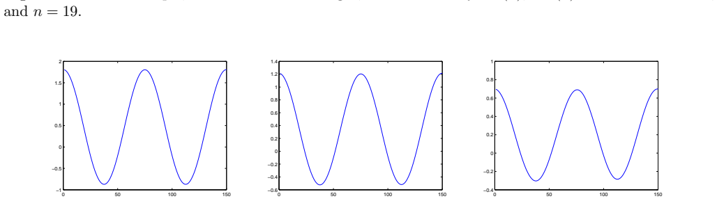
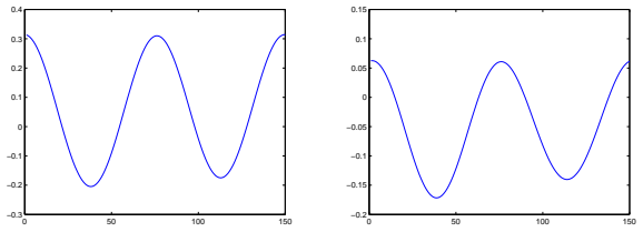
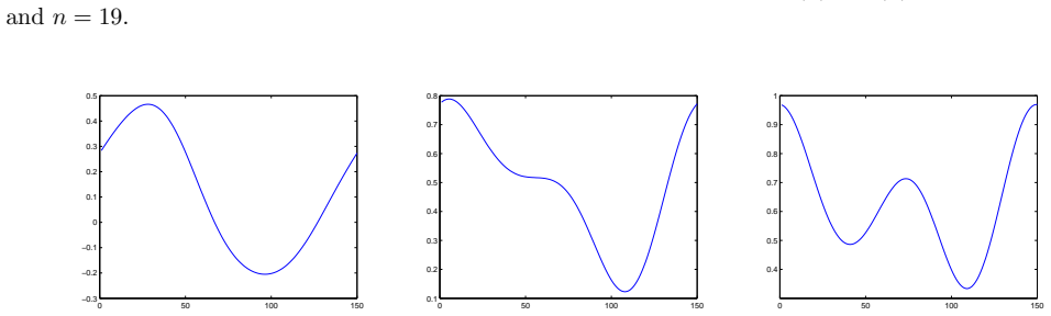
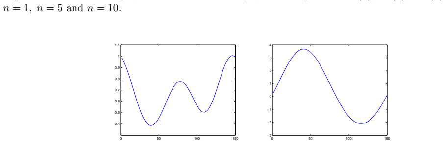
- [Figures 1-12] The figures would be more informative with labeled axes, since only the x-axis unit convention is supplied in the captions and no comparison with a known solution is shown.
- [Line 9, v9 formula] In the v9 expression, the coefficients −0.057 f6 u0 v0′ and −0.057 f8 v0 v0′ appear inconsistent with the monotone coefficient progression in neighboring lines; this may be a typographical error.
Circularity Check
Numerical validation is circular: the coefficients are least-squares fits to J, and the small minimized J is then cited as evidence of good approximations.
-
fitted input called prediction
[Section 3.1, numerical examples, after Eqs. (26)-(29)]
"as, above mentioned, the coefficients {ai[n]}, {bi[n]}, {ci[n]} have been obtained through the numerical minimization of J({un}, {vn}, {Pn}), so that for the mesh in question, we have obtained For this first example: J({un}, {vn}, {Pn}) ≈ 9.23 10−12 ... For this second example: J({un}, {vn}, {Pn}) ≈ 6.0 ∗ 10−7 ... In any case, considering the values obtained for J, it seems we have got good first approximations for the concerning solutions."
The same functional J defined in (29) as the L2 residual of the Navier-Stokes equations is used twice: first as the objective minimized to determine the undetermined coefficients in the ansatz (26)-(28), and then as the reported evidence that the resulting fields are good approximations. A minimized in-sample residual is forced by the fitting procedure, so the 'good first approximations' conclusion is a restatement of the fit, not an independent prediction or validation.
full rationale
The paper's exact construction (Theorem 2.1) is not circular: it defines u,v through (7)-(8) and tries to recover P from a curl-free momentum residual. The proof's failure to justify single-valuedness of P on the annulus and the prescribed trace P=P0 on Γ1 is a correctness gap, not a self-referential derivation. The self-citations to earlier work on the generalized method of lines [2,4,5,6] are contextual and not load-bearing; the line expressions are stated in the paper itself. The central circularity is confined to the numerical section: coefficients are fitted by minimizing the residual functional J, and the resulting minimized value of the same J is then quoted to conclude the approximations are good. That conclusion is a tautology of the least-squares fit. Because this circular validation supports the numerical 'good first approximations' claim rather than the main exact theorem, the overall circularity score is 6 rather than higher.
Assumptions & free parameters
free parameters (2)
- Line expression coefficients a_i[n], b_i[n], c_i[n] =
reported as decimals (e.g., a_2[1] ≈ 0.899, c_1[1] ≈ 0.101)
- Regularization parameter ε in approximate system (25) =
not specified, described only as 'very small'
assumptions (5)
- domain assumption A curl-free vector field on the doubly connected domain Ω implies existence of a single-valued pressure P with prescribed trace P0 on Γ1.
- ad hoc to paper Boundary data u0, v0 are compatible with an irrotational velocity field (vorticity φ = 0 in Ω).
- ad hoc to paper The fixed point iteration for T_n is a contraction on a complete metric space.
- domain assumption The truncated series in d up to order d^2 gives a valid approximation for the chosen mesh.
- standard math Standard elliptic existence and regularity for the linear system (8) with the given boundary data.
Cite this review
Pith. "Pith review of On the generalized method lines applied to the time-independent incompressible Navier-Stokes system." pith.science (2026). https://pith.science/paper/TLINTBMT
@misc{pith2026190809751,
  author       = {Pith},
  title        = {Pith review of: On the generalized method lines applied to the time-independent incompressible Navier-Stokes system},
  year         = {2026},
  howpublished = {\url{https://pith.science/paper/TLINTBMT}},
  note         = {Machine review of arXiv:1908.09751}
}
read the original abstract
In the first part of this article, we obtain a linear system whose the solution solves the time-independent incompressible Navier-Stokes system for the special case in which the external forces vector is a gradient. In a second step we develop approximate solutions, also for the time independent incompressible Navier-Stokes system, through the generalized method of lines. We recall that for such a method, the domain of the partial differential equation in question is discretized in lines and the concerning solution is written on these lines as functions of the boundary conditions and boundary shape. Finally, we emphasize these last main results are established through applications of the Banach fixed point theorem.
Figures
Figures from the paper (9 more)
Reference graph
Works this paper leans on
-
[1]
R.A. Adams and J.F. Fournier, Sobolev Spaces, 2nd edn. El sevier, New York, 2003
work page 2003
-
[2]
F. Botelho, Topics on Functional Analysis, Calculus of V ariations and Duality, Academic Publications, Sofia, (2011). 19 0 50 100 150 −1.5 −1 −0.5 0 0.5 1 1.5 0 50 100 150 −1 −0.8 −0.6 −0.4 −0.2 0 0.2 0.4 0.6 0.8 1 0 50 100 150 −0.8 −0.6 −0.4 −0.2 0 0.2 0.4 0.6 Figure 7: Second example, from the left to the right, fields of velocity u1(x), u 5(x), u 10(x) f...
work page 2011
-
[3]
Botelho, Variational Convex Analysis, Lambert Acade mic Publishing, Berlin, June 2010
F. Botelho, Variational Convex Analysis, Lambert Acade mic Publishing, Berlin, June 2010
work page 2010
-
[4]
F. Botelho, Existence of solution for the Ginzburg-Landau system, a rel ated optimal control problem and its computation by the generalized method of lin es, Applied Mathematics and Computation, 218, 11976-11989, (2012)
work page 2012
-
[5]
Botelho, Functional Analysis and Applied Optimizati on in Banach Spaces, Springer Switzerland, 2014
F. Botelho, Functional Analysis and Applied Optimizati on in Banach Spaces, Springer Switzerland, 2014
work page 2014
-
[6]
F.Botelho, On the generalized method of lines and its pro ximal and hyper-finite difference 20 0 50 100 150 −0.3 −0.2 −0.1 0 0.1 0.2 0.3 0.4 0 50 100 150 −0.2 −0.15 −0.1 −0.05 0 0.05 0.1 0.15 Figure 10: Second example, from the left to the right, fields of velocity v15(x), v 19(x) for the lines n = 15, and n = 19. 0 50 100 150 −0.3 −0.2 −0.1 0 0.1 0.2 0.3 0....
-
[7]
J.C. Strikwerda, Finite Difference Schemes and Partial Differential Equation s, SIAM, sec- ond edition (2004)
work page 2004
-
[8]
Temam, Navier-Stokes Equations, AMS Chelsea, reprint (2001)
R. Temam, Navier-Stokes Equations, AMS Chelsea, reprint (2001). 21
work page 2001
Reviewed August 14, 2026 · model on record in the stance chip above.
Discussion (0). Continue with ORCID to comment.