REVIEW 2 major objections 4 minor 64 references
Low multipole mapmaking for global 21-cm experiments
T0 review · 2 major / 4 minor · reviewed 2026-08-06 · deepseek-v4-flash
Pith's one-line read A CMB-style mapmaking inversion can recover the 21-cm global signal from chromatic-beam data that break standard foreground fits.
desk verdict Solid methods paper: CMB-style GLS mapmaking for global 21-cm works when the high-ℓ foreground mean/covariance are right, but the robustness claim is tested only against scatter, not bias. read the letter →
The pith
A machine-rendered reading of the paper's core claim, the machinery that carries it, and where it could break.
The reading
What carries the argument
The load-bearing object is the linear observation equation $d = G P Y B a + n$, where $B$ encodes the azimuthally symmetric beam as spherical-harmonic coefficients, $Y$ maps coefficients to pixels, $P$ is the pointing matrix of a latitudinally separated antenna array, and $G$ bins the time-ordered data. The method inverts this equation with the generalized least-squares estimator $\hat{a}' = W'(d - A''\mu'')$, where the covariance matrix $C = S + N$ includes both noise and the uncertainty in the higher-order modes. The mean $\mu''$ and covariance $C''_a$ of the corrected modes come from a stochastic 2-basemap extrapolation (S2BE) model: Gaussian deviations are added to the spectral index of every pixel, so the fractional pixel error is roughly Gaussian at the percent level, and the covariance propagates analytically through the spherical-harmonic transform.
What would settle it
Generate mock observations from a foreground sky whose high-$\ell$ modes have the same mean and covariance as the S2BE prior but are drawn from a non-Gaussian or spatially correlated distribution, or whose mean is shifted by a 10\% calibration error in the 408 MHz base map, then run the mapmaking pipeline with the unmodified S2BE prior and check whether the recovered 21-cm amplitude and width remain within $1\sigma$ of the injected values.
Extended reading notes
Core claim
The central claim is that the beam-chromatic foreground coupling that biases single-spectrum fits is removable in advance: a global 21-cm experiment can estimate the chromaticity-free low-$\ell$ sky modes, including the monopole, by inverting the observation equation with generalized least squares. The inversion is under-determined for high-$\ell$ modes because the beams are broad and the antennas fixed, so the method subtracts $A''\mu''$ from the data and inflates the noise covariance by $S = A''C''_a A''^T$, using only the mean and covariance of modes above $\ell_{\mathrm{mod}} = 5$. With these two inputs, the recovered monopole is fit by a smooth log-polynomial foreground and a Gaussian 21-cm model. The paper demonstrates that for chromatic beams with curvature $c = 1.6 \times 10^{-2}$ and $3.4 \times 10^{-2}$, the method recovers the injected 21-cm signal to $1\sigma$ with 10\% foreground-correction error, where the BFCC single-spectrum fit fails; even at $c = 5.2 \times 10^{-2}$ the signal is recovered, while 20\% correction error widens the posterior and weakens the detection.
Load-bearing premise
The load-bearing premise is that the mean and covariance of the high-order foreground modes ($\ell > 5$) are known and that the true high-$\ell$ foregrounds are a Gaussian draw from that distribution; in the paper's simulations the correction is built from the exact S2BE model that generated the data, so a systematically biased or structurally different prior is never tested.
Editorial extensions
If this is right
- For chromatic beams up to $c = 3.4 \times 10^{-2}$, the mapmaking monopole yields unbiased 21-cm posteriors at 10\% foreground-correction error, while the BFCC single-spectrum fit yields posteriors consistent with no signal or spanning roughly 50 to 850 mK.
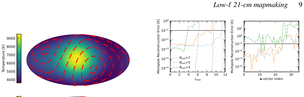
- With a 7-antenna latitudinally separated array, low-order modes up to $\ell_{\mathrm{mod}} = 5$ can be reconstructed with monopole error near the 2 mK noise floor, and the recovered monopole can be fit with a 3-term log-polynomial.
- The method requires only the mean and covariance of $\ell > 5$ foreground modes, not an exact foreground template, so a calibrated probabilistic foreground model with error propagation could supply these for real data.
- At 20\% foreground-correction error the recovered 21-cm signal is still inferred at $2\sigma$, but the posterior is broad enough that it would be difficult to distinguish from unknown systematics.
- The same observation-equation formalism extends to non-azimuthally symmetric beams, antennas with different beam profiles, and pointable or satellite-based instruments without changing the mapmaking inversion.
Reading between the lines
- If the approach transfers to real instruments, the natural first validation is on data from existing latitudinally separated sites, where beam calibration errors, assumed perfect here, will be the dominant new uncertainty.
- The 10\% tolerance probably depends on the Gaussianity of the high-$\ell$ modes; a prior with the same mean and covariance but heavier tails or spatial correlations could bias the monopole estimate more than the quoted 10\%.
- A satellite-based or steerable full-sky scanning experiment would remove the need for the high-$\ell$ prior entirely, since every mode would be observed; the same observation-equation formalism would apply unchanged.
- The method could be combined with training-set foreground models to absorb beam uncertainty, since the mapmaking inversion currently assumes the beam spherical harmonics are known exactly.
Editorial analysis
A structured set of objections, weighed in public.
Referee Report
Summary. The paper presents a mapmaking-based method for extracting the sky-averaged 21-cm signal from global 21-cm experiments. The authors write the beam-weighted observation of the sky by multiple latitudinally separated antennas as a linear observation equation, invert it with generalized least squares to estimate low-order spherical harmonics (ℓ ≲ 5), and correct for higher-order modes using a known mean and covariance of a stochastic foreground model. They benchmark the method against a single-spectrum fit with beam-factor chromaticity correction (BFCC), showing that BFCC fails for chromatic beams while the mapmaking method recovers the injected 21-cm signal when the higher-mode foreground correction has 10% scatter. The method is demonstrated on controlled simulations in which the sky is a realization of the same S2BE model whose mean and covariance provide the correction.
Significance. If the result holds, the paper offers a conceptually new route to mitigating beam-chromatic foreground coupling in global 21-cm experiments: instead of requiring an accurate foreground template, it uses a probabilistic description of high-ℓ foreground modes. The GLS derivation is standard and correct, the S2BE mean and covariance are derived analytically in Appendix A, and the code is made publicly available. The comparison with BFCC is useful and fairly constructed. The main limitation, correctly identified by the authors in the abstract and Section 6.2, is that the method assumes the mean and covariance of high-ℓ foreground modes are known; the demonstrations are self-consistent in the sense that the same model generates the sky and provides the correction. This makes the headline '10% uncertainty' claim conditional on the correction being correctly centered as well as correctly covarianced, a point that deserves explicit stress testing before the method can be taken as robust in realistic settings.
major comments (2)
- [Sections 5.3-5.4, Eqs. (27)-(29)] The 10%-error demonstrations are matched-filter tests: the sky is generated from the S2BE model and the correction uses the exact analytic mean μ″ and covariance C″_a of that same model. A biased correction mean, for example from base-map calibration errors of order 10-60% as cited in Section 5, would enter Eq. (26) as the deterministic leakage term W′A″(μ″_true − μ″_wrong), which is not controlled by the covariance S. Since Section 5.1 shows that uncorrected high-ℓ modes can bias the monopole at the ~K level, this leakage could easily exceed the ~20 mK posterior width reported in Fig. 8. The paper should include simulations with a systematically biased μ″ (e.g., a spectral-index offset or an independent foreground model) and report the resulting monopole bias and posterior coverage; without such a test, the statement that the method succeeds with 'uncertainty at the 10% level' is only supported for correctly centered scatter.
- [Section 6.2] The paper acknowledges that non-Gaussian high-ℓ modes would break the optimality of the GLS inversion, but no non-Gaussian or structurally different foreground model is tested. The S2BE model produces approximately Gaussian Δ″ by construction, as shown in Eq. (31), so the simulations never exercise the regime where the assumed Gaussian likelihood is misspecified. A concrete test with a non-Gaussian foreground residual (or a foreground model with spatial correlations not captured by the diagonal pixel covariance) would quantify how much degradation actually occurs and whether the method remains usable at the claimed 10% error level.
minor comments (4)
- [Section 3.2.3] The sentence 'the length scale of each pixel must be greater than the size of the smallest angular scale represented by lmax' should read 'smaller than'; the subsequent justification (NSIDE=32 gives a pixel width about 3 times smaller than the lmax=32 scale) is consistent with the corrected wording.
- [Section 3.2.3] The phrase 'approximately an order of 5 smaller' appears to be a typo; from the context and Fig. 2, the residual at lmax=32 is about an order of magnitude smaller than the 21-cm signal, not five orders of magnitude.
- [Fig. 10 caption] The caption refers to 'c = 3.2 × 10⁻²' but the corresponding cases in the text and Fig. 8 use c = 3.4 × 10⁻²; the values should be made consistent.
- [Fig. 10 caption] The phrase 'the three right-hand cases in Figs. 7 to 9' is unclear; it should specify the exact panels (e.g., Fig. 7 right, Fig. 8 right, Fig. 9 right).
Circularity Check
No circularity: the 21-cm signal is injected independently and never used to build the high-ell foreground correction; the GLS covariance is an assumed input, not a fitted parameter reused as a prediction.
full rationale
The derivation chain is not circular. The S2BE foreground model is used both to generate the mock sky and to construct the mean mu'' and covariance C''_a of the high-ell modes (Eqs. 28-29, Appendix A); the GLS estimator (Eq. 26) then uses these as assumed inputs, exactly as a CMB mapmaker uses a noise covariance. The 21-cm signal is added separately (Eq. 14, Section 2.1) and is never used to set mu'', C''_a, or S; it is only recovered by the final single-spectrum fit. No parameter is fitted to the data and then re-used as a prediction: the recovered monopole is fit with a log-polynomial plus the 21-cm model, and the 21-cm parameters are the output. The only caveat is that the simulations are self-consistent: the correction mean and covariance coincide with the generative model, and non-Gaussian or biased high-ell modes are not exercised (Section 6.2). This is a validation limitation and a robustness risk, but it is not circularity: the mapmaking success is not equivalent by construction to the assumptions, because the 21-cm inference step is a non-trivial fit to noisy data and could in principle fail even with a correct foreground covariance. Citations to the authors' prior work (e.g., Ignatov et al. 2024 for dipole information) are not load-bearing here; the need for multiple antennas is also demonstrated directly in Fig. 5. No specific circular step can be quoted.
Assumptions & free parameters
free parameters (3)
- sigma_delta (equiv. sigma_T at 70 MHz) =
0.057 (10%), 0.11 (20%)
- l_mod =
5
- N_ant =
7
assumptions (5)
- domain assumption The antenna beam is azimuthally symmetric.
- ad hoc to paper The high-l (l > l_mod) foreground modes are Gaussian with known mean and covariance.
- domain assumption The 21-cm signal is a pure monopole.
- domain assumption Noise is Gaussian, independent, with radiometer equation variance from Eq. (11).
- ad hoc to paper The true foreground sky is a realization of the S2BE model used for correction.
Cite this review
Pith. "Pith review of Low multipole mapmaking for global 21-cm experiments." pith.science (2026). https://pith.science/paper/TRV5HNNV
@misc{pith2026250621258,
  author       = {Pith},
  title        = {Pith review of: Low multipole mapmaking for global 21-cm experiments},
  year         = {2026},
  howpublished = {\url{https://pith.science/paper/TRV5HNNV}},
  note         = {Machine review of arXiv:2506.21258}
}
abstract
The 21-cm global signal is obscured by very bright galactic and extra galactic foreground emissions. Typical single-spectrum fit (SSF) based methods for foreground/signal separation can result in biased estimates of the cosmological signal due to the presence of spectral oscillations induced by the interaction between chromatic beams and the spatial shape of the foregrounds. Modelling this interaction requires some amount of assumed foreground information. We present a mapmaking-based approach which describes the beam-weighted observation of the sky by multiple globally-distributed antenna experiments as an observation equation. This equation is inverted in order to estimate the low-order sky modes ($\ell\lesssim10$). The resulting chromaticity-free sky monopole is then fit with a smooth foreground function and a 21-cm model. Given the insensitivity of global 21-cm experiments to small angular scales, we rely on the mean and covariance of higher-order foreground modes being known. We show that this mapmaking-based method is capable of inferring the cosmological signal in cases where a SSF with a simple beam-factor based chromaticity correction fails, even when the foreground model used in the mapmaking method features uncertainty at the 10\% level.
Figures


Figures from the paper (6 more)


Reference graph
Works this paper leans on
-
[1]
Anstey D., de Lera Acedo E., Handley W., 2021, @doi [ ] 10.1093/mnras/stab1765 , https://ui.adsabs.harvard.edu/abs/2021MNRAS.506.2041A 506, 2041
-
[2]
Anstey D., de Lera Acedo E., Handley W., 2023, @doi [ ] 10.1093/mnras/stad156 , https://ui.adsabs.harvard.edu/abs/2023MNRAS.520..850A 520, 850
-
[3]
Barkana R., 2018, @doi [ ] 10.1038/nature25791 , 555, 71
-
[4]
Barrett J., Cappallo R., Soohoo J., 2025, EDGES Memo 396, MIT Haystack Observatory, https://dspace.mit.edu/bitstream/handle/1721.1/154786/memo_EDGES_396.pdf
work page 2025
-
[5]
J., 2015, @doi [ ] 10.1088/0004-637x/799/1/90 , 799, 90
Bernardi G., McQuinn M., Greenhill L. J., 2015, @doi [ ] 10.1088/0004-637x/799/1/90 , 799, 90
-
[6]
Bowman J. D., Rogers A. E. E., Monsalve R. A., Mozdzen T. J., Mahesh N., 2018, @doi [ ] 10.1038/nature25792 , https://ui.adsabs.harvard.edu/abs/2018Natur.555...67B 555, 67
-
[7]
Brandenberger R., Cyr B., Shi R., 2019, @doi [JCAP] 10.1088/1475-7516/2019/09/009 , https://ui.adsabs.harvard.edu/abs/2019JCAP...09..009B 2019, 009
-
[8]
Bull P., et al., 2024, @doi [arXiv e-prints] 10.48550/arXiv.2410.00076 , https://ui.adsabs.harvard.edu/abs/2024arXiv241000076B p. arXiv:2410.00076
Show all 64 references
-
[9]
O., 2021, @doi [Philosophical Transactions of the Royal Society of London Series A] 10.1098/rsta.2019.0564 , https://ui.adsabs.harvard.edu/abs/2021RSPTA.37990564B 379, 20190564
Burns J. O., 2021, @doi [Philosophical Transactions of the Royal Society of London Series A] 10.1098/rsta.2019.0564 , https://ui.adsabs.harvard.edu/abs/2021RSPTA.37990564B 379, 20190564
2021
-
[10]
C., Barrett J
Cappallo R. C., Barrett J. P., 2025, EDGES Memo 470, MIT Haystack Observatory, https://www.haystack.mit.edu/wp-content/uploads/2025/01/EDGES-MEMO_470.pdf
2025
-
[11]
Carter G., Handley W., Ashdown M., Razavi-Ghods N., 2025, @doi [arXiv e-prints] 10.48550/arXiv.2501.01417 , https://ui.adsabs.harvard.edu/abs/2025arXiv250101417C
2025 doi
-
[12]
Chen X., Yan J., Deng L., Wu F., Wu L., Xu Y., Zhou L., 2021, @doi [Philosophical Transactions of the Royal Society of London Series A] 10.1098/rsta.2019.0566 , https://ui.adsabs.harvard.edu/abs/2021RSPTA.37990566C 379, 20190566
2021
-
[13]
Cohen A., Fialkov A., Barkana R., Lotem M., 2017, @doi [ ] 10.1093/mnras/stx2065 , https://ui.adsabs.harvard.edu/abs/2017MNRAS.472.1915C 472, 1915
2017 doi
-
[14]
A., 2018, @doi [ ] 10.3847/2041-8213/aae318 , https://ui.adsabs.harvard.edu/abs/2018ApJ...866L...7D 866, L7
Deshpande A. A., 2018, @doi [ ] 10.3847/2041-8213/aae318 , https://ui.adsabs.harvard.edu/abs/2018ApJ...866L...7D 866, L7
2018 doi
-
[15]
B., Schinzel F
Dowell J., Taylor G. B., Schinzel F. K., Kassim N. E., Stovall K., 2017, @doi [ ] 10.1093/mnras/stx1136 , https://ui.adsabs.harvard.edu/abs/2017MNRAS.469.4537D 469, 4537
2017 doi
-
[16]
B., 1958, @doi [Proc
Field G. B., 1958, @doi [Proc. IRE] 10.1109/JRPROC.1958.286741 , https://ui.adsabs.harvard.edu/abs/1958PIRE...46..240F 46, 240
1958
-
[17]
W., Lang D., Goodman J., 2013, @doi [ ] 10.1086/670067 , https://ui.adsabs.harvard.edu/abs/2013PASP..125..306F 125, 306
Foreman-Mackey D., Hogg D. W., Lang D., Goodman J., 2013, @doi [ ] 10.1086/670067 , https://ui.adsabs.harvard.edu/abs/2013PASP..125..306F 125, 306
2013 doi
-
[18]
Fraser S., et al., 2018, @doi [Phys. Lett. B] 10.1016/j.physletb.2018.08.035 , https://ui.adsabs.harvard.edu/abs/2018PhLB..785..159F 785, 159
2018 doi
-
[19]
Haslam C. G. T., Salter C. J., Stoffel H., Wilson W. E., 1982, , https://ui.adsabs.harvard.edu/abs/1982A&AS...47....1H 47, 1
1982
-
[20]
D., Puchwein E., 2018, @doi [ ] 10.1038/s41586-018-0796-5 , https://ui.adsabs.harvard.edu/abs/2018Natur.564E..32H 564, E32
Hills R., Kulkarni G., Meerburg P. D., Puchwein E., 2018, @doi [ ] 10.1038/s41586-018-0796-5 , https://ui.adsabs.harvard.edu/abs/2018Natur.564E..32H 564, E32
2018 doi
-
[21]
C., Ahn K., 2024, @doi [ ] 10.3847/1538-4357/ad2209 , https://ui.adsabs.harvard.edu/abs/2024ApJ...964...21H 964, 21
Hotinli S. C., Ahn K., 2024, @doi [ ] 10.3847/1538-4357/ad2209 , https://ui.adsabs.harvard.edu/abs/2024ApJ...964...21H 964, 21
2024 doi
-
[22]
D., Pritchard J
Ignatov Y. D., Pritchard J. R., Wu Y., 2024, @doi [ ] 10.1093/mnras/stad3931 , https://ui.adsabs.harvard.edu/abs/2024MNRAS.52711206I 527, 11206
2024 doi
- [23]
-
[24]
Keih \"a nen E., et al., 2023, @doi [ ] 10.1051/0004-6361/202142799 , https://ui.adsabs.harvard.edu/abs/2023A&A...675A...2K 675, A2
2023 doi
-
[25]
Mirocha J., 2014, @doi [ ] 10.1093/mnras/stu1193 , https://ui.adsabs.harvard.edu/abs/2014MNRAS.443.1211M 443, 1211
2014 doi
-
[26]
R., 2019, @doi [ ] 10.1093/mnras/sty3260 , https://ui.adsabs.harvard.edu/abs/2019MNRAS.483.1980M 483, 1980
Mirocha J., Furlanetto S. R., 2019, @doi [ ] 10.1093/mnras/sty3260 , https://ui.adsabs.harvard.edu/abs/2019MNRAS.483.1980M 483, 1980
2019 doi
-
[27]
Mirocha J., Anderson C., Chang T.-C., Dor \'e O., Lidz A., 2025, @doi [ ] 10.3847/1538-4357/adbdce , https://ui.adsabs.harvard.edu/abs/2025ApJ...983...54M 983, 54
2025 doi
-
[28]
Mittal S., Kulkarni G., 2022, @doi [ ] 10.1093/mnras/stac1961 , https://ui.adsabs.harvard.edu/abs/2022MNRAS.515.2901M 515, 2901
2022 doi
-
[29]
A., et al., 2024a, @doi [ ] 10.1093/mnras/stae1138 , https://ui.adsabs.harvard.edu/abs/2024MNRAS.530.4125M 530, 4125
Monsalve R. A., et al., 2024a, @doi [ ] 10.1093/mnras/stae1138 , https://ui.adsabs.harvard.edu/abs/2024MNRAS.530.4125M 530, 4125
-
[30]
A., et al., 2024b, @doi [ ] 10.3847/1538-4357/ad0f1b , https://ui.adsabs.harvard.edu/abs/2024ApJ...961...56M 961, 56
Monsalve R. A., et al., 2024b, @doi [ ] 10.3847/1538-4357/ad0f1b , https://ui.adsabs.harvard.edu/abs/2024ApJ...961...56M 961, 56
-
[31]
J., Bowman J
Mozdzen T. J., Bowman J. D., Monsalve R. A., Rogers A. E. E., 2016, @doi [ ] 10.1093/mnras/stv2601 , https://ui.adsabs.harvard.edu/abs/2016MNRAS.455.3890M 455, 3890
2016 doi
-
[32]
J., Bowman J
Mozdzen T. J., Bowman J. D., Monsalve R. A., Rogers A. E. E., 2017, @doi [ ] 10.1093/mnras/stw2696 , https://ui.adsabs.harvard.edu/abs/2017MNRAS.464.4995M 464, 4995
2017 doi
-
[33]
J., Mahesh N., Monsalve R
Mozdzen T. J., Mahesh N., Monsalve R. A., Rogers A. E. E., Bowman J. D., 2019, @doi [ ] 10.1093/mnras/sty3410 , https://ui.adsabs.harvard.edu/abs/2019MNRAS.483.4411M 483, 4411
2019 doi
-
[34]
B., Loeb A., 2018, @doi [ ] 10.1038/s41586-018-0151-x , https://ui.adsabs.harvard.edu/abs/2018Natur.557..684M 557, 684
Mu \ n oz J. B., Loeb A., 2018, @doi [ ] 10.1038/s41586-018-0151-x , https://ui.adsabs.harvard.edu/abs/2018Natur.557..684M 557, 684
2018 doi
-
[35]
J., et al., 2021, Experimental Astronomy, https://ui.adsabs.harvard.edu/abs/2021arXiv210401756N 51, 193
Nambissan T. J., et al., 2021, Experimental Astronomy, https://ui.adsabs.harvard.edu/abs/2021arXiv210401756N 51, 193
2021
-
[36]
Pagano M., Sims P., Liu A., Anstey D., Handley W., de Lera Acedo E., 2024, @doi [ ] 10.1093/mnras/stad3392 , https://ui.adsabs.harvard.edu/abs/2024MNRAS.527.5649P 527, 5649
2024 doi
-
[37]
Philip L., et al., 2019, @doi [J. Astron. Instrum.] 10.1142/S2251171719500041 , https://ui.adsabs.harvard.edu/abs/2019JAI.....850004P 8, 1950004
2019 doi
-
[38]
T., Urbano A., 2018, @doi [ ] 10.1103/PhysRevLett.121.031103 , https://ui.adsabs.harvard.edu/abs/2018PhRvL.121c1103P 121, 031103
Pospelov M., Pradler J., Ruderman J. T., Urbano A., 2018, @doi [ ] 10.1103/PhysRevLett.121.031103 , https://ui.adsabs.harvard.edu/abs/2018PhRvL.121c1103P 121, 031103
2018 doi
-
[39]
C., et al., 2018, @doi [ ] 10.1093/mnras/sty1244 , https://ui.adsabs.harvard.edu/abs/2018MNRAS.478.4193P 478, 4193
Price D. C., et al., 2018, @doi [ ] 10.1093/mnras/sty1244 , https://ui.adsabs.harvard.edu/abs/2018MNRAS.478.4193P 478, 4193
2018 doi
-
[40]
R., Loeb A., 2012, @doi [Rep
Pritchard J. R., Loeb A., 2012, @doi [Rep. Prog. Phys.] 10.1088/0034-4885/75/8/086901 , https://ui.adsabs.harvard.edu/abs/2012RPPh...75h6901P 75, 086901
2012 doi
-
[41]
O., 2020, @doi [ ] 10.3847/1538-4357/ab9b29 , https://ui.adsabs.harvard.edu/abs/2020ApJ...897..174R 897, 174
Rapetti D., Tauscher K., Mirocha J., Burns J. O., 2020, @doi [ ] 10.3847/1538-4357/ab9b29 , https://ui.adsabs.harvard.edu/abs/2020ApJ...897..174R 897, 174
2020 doi
-
[42]
J., Bigot-Sazy M.-A., Ghosh T., 2015, @doi [MNRAS] 10.1093/mnras/stv1274 , 451, 4311
Remazeilles M., Dickinson C., Banday A. J., Bigot-Sazy M.-A., Ghosh T., 2015, @doi [MNRAS] 10.1093/mnras/stv1274 , 451, 4311
2015 doi
-
[43]
Sathyanarayana Rao M., et al., 2023, @doi [Experimental Astronomy] 10.1007/s10686-023-09909-5 , https://ui.adsabs.harvard.edu/abs/2023ExA....56..741S 56, 741
2023 doi
-
[44]
D., de Lera Acedo E., Handley W., Koopmans L
Saxena A., Meerburg P. D., de Lera Acedo E., Handley W., Koopmans L. V. E., 2023, @doi [ ] 10.1093/mnras/stad1047 , https://ui.adsabs.harvard.edu/abs/2023MNRAS.522.1022S 522, 1022
2023 doi
- [45]
-
[46]
R., Sigurdson K., Pen U.-L., Stebbins A., Sitwell M., 2014, @doi [ ] 10.1088/0004-637X/781/2/57 , https://ui.adsabs.harvard.edu/abs/2014ApJ...781...57S 781, 57
Shaw J. R., Sigurdson K., Pen U.-L., Stebbins A., Sitwell M., 2014, @doi [ ] 10.1088/0004-637X/781/2/57 , https://ui.adsabs.harvard.edu/abs/2014ApJ...781...57S 781, 57
2014 doi
-
[47]
Shi Y., Deng F., Xu Y., Wu F., Yan Q., Chen X., 2022, @doi [ ] 10.3847/1538-4357/ac5965 , https://ui.adsabs.harvard.edu/abs/2022ApJ...929...32S 929, 32
2022 doi
-
[48]
H., Pober J
Sims P. H., Pober J. C., 2020, @doi [ ] 10.1093/mnras/stz3388 , https://ui.adsabs.harvard.edu/abs/2020MNRAS.492...22S 492, 22
2020 doi
-
[49]
H., et al., 2023, @doi [MNRAS] 10.1093/mnras/stad610 , 521, 3273
Sims P. H., et al., 2023, @doi [MNRAS] 10.1093/mnras/stad610 , 521, 3273
2023 doi
-
[50]
Singh S., Subrahmanyan R., 2019, @doi [ApJ] 10.3847/1538-4357/ab2879 , 880, 26
2019 doi
-
[51]
Astron.] 10.1038/s41550-022-01610-5 , https://ui.adsabs.harvard.edu/abs/2022NatAs...6..607S 6, 607
Singh S., et al., 2022, @doi [Nat. Astron.] 10.1038/s41550-022-01610-5 , https://ui.adsabs.harvard.edu/abs/2022NatAs...6..607S 6, 607
2022 doi
-
[52]
V., eds, American Institute of Physics Conference Series Vol
Skilling J., 2004, in Fischer R., Preuss R., Toussaint U. V., eds, American Institute of Physics Conference Series Vol. 735, Bayesian Inference and Maximum Entropy Methods in Science and Engineering: 24th International Workshop on Bayesian Inference and Maximum Entropy Methods...
2004 doi
-
[53]
Slosar A., 2017, @doi [ ] 10.1103/PhysRevLett.118.151301 , https://ui.adsabs.harvard.edu/abs/2017PhRvL.118o1301S 118, 151301
2017 doi
-
[54]
J., Fialkov A., Garsden H., 2022, @doi [ ] 10.1093/mnras/stac1804 , https://ui.adsabs.harvard.edu/abs/2022MNRAS.515.1580S 515, 1580
Spinelli M., Kyriakou G., Bernardi G., Bolli P., Greenhill L. J., Fialkov A., Garsden H., 2022, @doi [ ] 10.1093/mnras/stac1804 , https://ui.adsabs.harvard.edu/abs/2022MNRAS.515.1580S 515, 1580
2022 doi
-
[55]
O., Switzer E., 2018, @doi [ ] 10.3847/1538-4357/aaa41f , https://ui.adsabs.harvard.edu/abs/2018ApJ...853..187T 853, 187
Tauscher K., Rapetti D., Burns J. O., Switzer E., 2018, @doi [ ] 10.3847/1538-4357/aaa41f , https://ui.adsabs.harvard.edu/abs/2018ApJ...853..187T 853, 187
2018 doi
-
[56]
O., 2020a, @doi [ ] 10.3847/1538-4357/ab9a3f , https://ui.adsabs.harvard.edu/abs/2020ApJ...897..132T 897, 132
Tauscher K., Rapetti D., Burns J. O., 2020a, @doi [ ] 10.3847/1538-4357/ab9a3f , https://ui.adsabs.harvard.edu/abs/2020ApJ...897..132T 897, 132
-
[57]
O., 2020b, @doi [ ] 10.3847/1538-4357/ab9b2a , https://ui.adsabs.harvard.edu/abs/2020ApJ...897..175T 897, 175
Tauscher K., Rapetti D., Burns J. O., 2020b, @doi [ ] 10.3847/1538-4357/ab9b2a , https://ui.adsabs.harvard.edu/abs/2020ApJ...897..175T 897, 175
-
[58]
Tegmark M., 1997, @doi [ ] 10.1086/310631 , https://ui.adsabs.harvard.edu/abs/1997ApJ...480L..87T 480, L87
1997 doi
-
[59]
D., G \'o rski K
Wandelt B. D., G \'o rski K. M., 2001, @doi [ ] 10.1103/PhysRevD.63.123002 , https://ui.adsabs.harvard.edu/abs/2001PhRvD..63l3002W 63, 123002
2001 doi
-
[60]
J., Irfan M
Wilensky M. J., Irfan M. O., Bull P., 2025, @doi [ ] 10.1093/mnras/staf668 , https://ui.adsabs.harvard.edu/abs/2025MNRAS.539.3122W 539, 3122
2025 doi
-
[61]
A., 1952, @doi [ ] 10.1086/106661 , https://ui.adsabs.harvard.edu/abs/1952AJ.....57R..31W 57, 31
Wouthuysen S. A., 1952, @doi [ ] 10.1086/106661 , https://ui.adsabs.harvard.edu/abs/1952AJ.....57R..31W 57, 31
1952 doi
-
[62]
Astron.] 10.1038/s41550-022-01709-9 , https://ui.adsabs.harvard.edu/abs/2022NatAs...6..984D 6, 984
de Lera Acedo E., et al., 2022, @doi [Nat. Astron.] 10.1038/s41550-022-01709-9 , https://ui.adsabs.harvard.edu/abs/2022NatAs...6..984D 6, 984
2022 doi
-
[63]
de Oliveira-Costa A., Tegmark M., 2006, @doi [ ] 10.1103/PhysRevD.74.023005 , https://ui.adsabs.harvard.edu/abs/2006PhRvD..74b3005D 74, 023005
2006 doi
-
[64]
M., Jonas J., Landecker T
de Oliveira-Costa A., Tegmark M., Gaensler B. M., Jonas J., Landecker T. L., Reich P., 2008, @doi [ ] 10.1111/j.1365-2966.2008.13376.x , https://ui.adsabs.harvard.edu/abs/2008MNRAS.388..247D 388, 247
2008
Reviewed August 6, 2026 · model on record in the stance chip above.
Discussion (0). Continue with ORCID to comment.