REVIEW 3 major objections 5 minor 34 references
Fast Non-Line-of-Sight Transient Data Simulation and an Open Benchmark Dataset
T0 review · 3 major / 5 minor · reviewed 2026-08-07 · deepseek-v4-flash
Pith's one-line read A single depth map accurately simulates hidden-scene transient data for non-line-of-sight imaging.
desk verdict A practical simulator paper whose discrete PSF contradicts its own LCT derivation, so the dataset and benchmark inherit the error. read the letter →
The pith
A machine-rendered reading of the paper's core claim, the machinery that carries it, and where it could break.
The reading
What carries the argument
The central mechanism is the discretized light-cone transform (LCT) expressed as $\tau = R_t^{-1}\{ R_z(p) * \text{PSF} \}$, where $p$ is the albedo-weighted depth map volume, $R_z$ resamples the depth axis via a square-root mapping with amplitude normalization, $R_t^{-1}$ rescales the temporal axis by $v^{3/2}$, and PSF is a Boolean tensor representing the conical wavefront on a uniform grid. A slope parameter ties lateral spatial distances to axial time-depth coordinates, and multilevel binary down-sampling keeps the spatio-temporal coupling scale aligned with resolution, allowing the whole operation to run as a single FFT-accelerated convolution.
What would settle it
Compare the simulator's output against real confocal NLOS measurements taken on a laboratory scene whose geometry and surface reflectance are independently calibrated; if the simulated temporal profile or the shape reconstructed from it diverges beyond the modeled noise, the forward model is not adequate.
Extended reading notes
Core claim
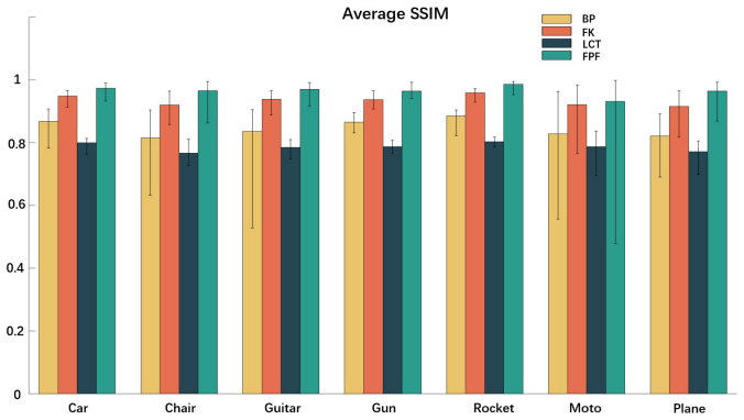
The paper demonstrates that the confocal NLOS transient measurement can be reduced to a three-dimensional convolution between a volume built from a depth map and a conical point-spread function (PSF), with two resampling operators that fold the depth axis and then unfold the temporal axis while conserving energy. The entire simulation pipeline takes a depth and albedo map as input, maps them to a voxel field, applies the FFT-based convolution, and then adds temporal jitter and Poisson noise, all with a parameter interface for system geometry and detector properties. Systematic experiments on seven ShapeNet categories show that the simulated transients, reconstructed by LCT, phasor field, f-k migration, and filtered backprojection, recover the original hidden shapes with high PSNR and SSIM, thereby validating the physical consistency of the synthetic data.
Load-bearing premise
That a single orthographic depth map with uniform Lambertian albedo, processed through the confocal light-cone transform, adequately represents what a real NLOS detector would record.
Editorial extensions
If this is right
- Researchers can generate custom NLOS transient datasets on demand for any depth map by adjusting wall size, stand-off distance, time bin, jitter, and noise, eliminating the need to modify shaders or scene files.
- Supervised deep-learning models for NLOS reconstruction can be trained on a large, physically consistent corpus covering diverse object classes and noise conditions, potentially enabling cross-hardware generalization.
- The released benchmark tables give a unified, reproducible baseline for comparing new reconstruction algorithms against LCT, phasor field, f-k migration, and filtered backprojection on the same data.
- System design can be optimized in software by sweeping detector time resolution, scan area, and noise parameters before committing to expensive hardware.
- Because the framework lowers the storage cost from a full volume to a depth map, large-scale batch processing of synthetic transients becomes practical for training purposes.
Reading between the lines
- The same discretized convolution could be inverted analytically to yield a fast reconstruction algorithm that is directly matched to the forward model, potentially outperforming the four generic baselines on the simulated data.
- The uniform Lambertian albedo assumption could be relaxed by extending the depth map input to a per-pixel BRDF or a small set of albedo channels, allowing simulation of more realistic surface finishes at little extra cost.
- The benchmark's synthetic-to-real gap could be tested by fine-tuning a network on these simulated transients and evaluating it on real experimental NLOS measurements; such a transfer test would be a natural next validation.
- The parameterized noise model (Gaussian jitter plus Poisson corruptions) could be used to study how reconstruction accuracy degrades as a function of time resolution or photon count, yielding design guidance for future SPAD systems.
Editorial analysis
A structured set of objections, weighed in public.
Referee Report
Summary. The manuscript proposes a fast NLOS transient simulator built on the light-cone transform (LCT). A depth map and optional albedo map are converted into a voxel field, resampled along depth, convolved in the Fourier domain with a discretized point-spread function, and then degraded by temporal Gaussian blur and Poisson noise. The authors release synthetic transients for seven ShapeNet object classes and report reconstruction SSIM/PSNR for LCT, phasor-field (PF), f-k migration (FK), and filtered backprojection (FBP). The central claim is that the simulator generates physically consistent transient measurements and that the released dataset provides a reproducible benchmark for NLOS reconstruction algorithms.
Significance. If the implementation were correct, the paper would offer a useful low-barrier tool: it requires only a depth map, exposes a compact parameter interface, and uses FFT acceleration, which is a practical advantage over path-tracing simulators. The release of a dataset and a comparison of four classical reconstruction algorithms is also potentially valuable for reproducible research. However, the physical-consistency claim currently rests on an internally generated benchmark with no independent validation, and the discrete PSF in the implementation does not match the continuous LCT derivation. The central contribution is therefore not yet established. With the kernel corrected and validation against an independent renderer or real data added, the tool and dataset could be a helpful resource, but the present version overstates its physical fidelity.
major comments (3)
- [Section 2 / Algorithm 1] The implemented PSF is internally inconsistent with the continuous LCT model. The continuous derivation uses u=z^2 and v=(ct/2)^2 and yields a kernel delta((x'-x)^2+(y'-y)^2+u-v), i.e. z^2 + (x'-x)^2 + (y'-y)^2 = (ct/2)^2. Algorithm 1, step 1.2, however, constructs PSF(x,y,z)=delta_K(|z - (16w^2/(c^2 T_max^2))(x^2+y^2)|, 0), which is a paraboloid in linear depth. The text's justification, 'Squaring this expression yields the form above', is algebraically incorrect: squaring z=(4/slope)r gives z^2=(4/slope)^2 r^2, not z=(4/slope)^2 r^2. Consequently, off-axis scene points are assigned temporal depths that do not satisfy the physical round-trip relation t=2*sqrt(r^2+z^2)/c. Since the released dataset and the scores in Tables 1-2 are produced with this kernel, the reported reconstructions validate only the self-consistency of the implementation, not the LCT forward model.
- [Section 3 / Tables 1-2] The experimental validation is circular. The transient data are generated with the LCT-based forward model, and the compared algorithms—especially LCT but also PF, FK, and FBP—are derived from the same wave-based light-cone model. No real measured transients, no independent Monte Carlo path tracer, and no withheld physical validation are used. Therefore the PSNR and SSIM values in Tables 1-2 demonstrate that the simulators and the inverses are mutually consistent, not that hidden geometries are accurately recovered from physically realistic NLOS measurements. The claim in the abstract and conclusion that reconstructions 'accurately recover hidden geometries' is not supported; an evaluation against an independent transient renderer or real experimental data is required.
- [Section 3] The use of a single orthographic depth map to represent the hidden object is a significant modeling limitation that is not discussed. NLOS transients integrate contributions from all surfaces visible from the relay wall, including multiple depth layers and self-occlusions, whereas an orthographic projection captures only one 2.5D view. Combined with the uniform Lambertian albedo of 1 used for the ShapeNet dataset, this restricts the diversity and realism of the benchmark. The claim that the corpus is 'physically consistent, diverse' is therefore overstated; the paper should disclose these simplifications and justify that they do not bias algorithm rankings.
minor comments (5)
- [Table 2] The header of Table 2 uses 'BP' for the filtered-backprojection row, while the text and Table 1 use 'FBP'; these labels should be made consistent.
- [Section 2 / Section 3] Section 2 defines a grid of (2N)x(2N)x(2M) nodes, while Section 3 describes a 128x128x1024 space-time grid; the relation between these dimensions is not explained and should be clarified.
- [Section 7] The Data availability section refers to 'Data Repository' and 'Code Repository' but gives no URLs or persistent identifiers, which prevents readers from accessing the claimed release.
- [Section 2] The definitions of the resampling operators R_z and R_t^{-1} are ambiguous: the row/column domains of R_z are not specified, and R_t^{-1}=R_z^T D_v^{3/2} refers to D_v of size M^2 while the preceding grid has 2M depth nodes. A complete index convention and a verification of energy conservation would make the derivation reproducible.
- [Section 2] The depth coordinate is mapped to the interval [-1,1], but physical depth is nonnegative; using a signed depth in the PSF and in the depth-to-volume mapping creates potential confusion about where the hidden surface is located.
Circularity Check
No significant circularity: the LCT-based simulator and benchmark are not equivalent by construction, since independent algorithms (PF, FK, FBP) outperform LCT on the synthetic data.
full rationale
The paper's chain is: (1) adopt the LCT forward model from O'Toole et al. [2]; (2) discretize it via resampling operators and FFT convolution; (3) generate transients from ShapeNet depth maps; (4) benchmark four reconstruction algorithms. The adopted forward model is not an input of the benchmark in a way that forces the results: the dataset is generated by the simulator, and the benchmarked methods include PF, FK, and FBP, which are independent algorithms developed outside this work and cited to external groups [2,17,33,34]. The tables show PF highest and LCT lowest, so the benchmark does not reduce to inverting the generator. The only self-referential aspect is that the same LCT model appears on both sides, but LCT is not the claimed output or the best performer, and no parameter is fitted to make a particular method succeed. The claim that reconstructions recover hidden geometries is an internal consistency check of the simulator, not a derivation of physics from the model. No prediction is renamed from a fit, and no load-bearing premise rests on self-citations. Note: the discrete PSF expression in Section 2/Algorithm 1 may be internally inconsistent with the continuous change-of-variables kernel (squared-depth vs linear-depth paraboloid), but that is a correctness issue and does not make the derivation circular.
Assumptions & free parameters
free parameters (4)
- slope =
w/(M c Δt)
- n_r (λ_poisson) =
2 (dataset default)
- temporal jitter FWHM =
70 ps (dataset default)
- uniform albedo =
1.0 (dataset default)
assumptions (6)
- domain assumption The confocal LCT forward model adequately represents real NLOS transient measurements
- domain assumption Hidden objects are Lambertian and light transport is single-bounce (wall-object-wall only)
- domain assumption An orthographic first-surface depth map and a flat albedo map fully describe the hidden scene for simulation purposes
- domain assumption Detector jitter is zero-mean Gaussian and independent per wall position
- standard math Photon counts follow Poisson statistics with variance equal to mean
- standard math Change of variables z=√u and the 3D convolution theorem via FFT are valid
Cite this review
Pith. "Pith review of Fast Non-Line-of-Sight Transient Data Simulation and an Open Benchmark Dataset." pith.science (2026). https://pith.science/paper/TSRNSPOB
@misc{pith2026250603747,
  author       = {Pith},
  title        = {Pith review of: Fast Non-Line-of-Sight Transient Data Simulation and an Open Benchmark Dataset},
  year         = {2026},
  howpublished = {\url{https://pith.science/paper/TSRNSPOB}},
  note         = {Machine review of arXiv:2506.03747}
}
read the original abstract
Non-Line-of-Sight (NLOS) imaging reconstructs the shape and depth of hidden objects from picosecond-resolved transient signals, offering potential applications in autonomous driving, security, and medical diagnostics. However, current NLOS experiments rely on expensive hardware and complex system alignment, limiting their scalability. This manuscript presents a simplified simulation method that generates NLOS transient data by modeling light-intensity transport rather than performing conventional path tracing, significantly enhancing computational efficiency. All scene elements, including the relay surface, hidden target, stand-off distance, detector time resolution, and acquisition window are fully parameterized, allowing for rapid configuration of test scenarios. Reconstructions based on the simulated data accurately recover hidden geometries, validating the effectiveness of the approach. The proposed tool reduces the entry barrier for NLOS research and supports the optimization of system design.
Figures


Figures from the paper (4 more)



Reference graph
Works this paper leans on
-
[1]
D. Faccio, A. Velten, and G. Wetzstein, “Non-line-of-sight imaging,” Nat. Rev. Phys.2, 318–327 (2020)
work page 2020
-
[2]
Confocalnon-line-of-sightimagingbasedonthelight-conetransform,
M.O’Toole,D.B.Lindell, andG.Wetzstein,“Confocalnon-line-of-sightimagingbasedonthelight-conetransform,” Nature555, 338–341 (2018)
work page 2018
-
[3]
Non-line-of-sightimagingwithpartial occluders and surface normals,
F.Heide, M.O’Toole, K.Zang, D.B.Lindell, S.Diamond, andG.Wetzstein, “Non-line-of-sightimagingwithpartial occluders and surface normals,” ACM Trans. on Graph. (ToG)38, 1–10 (2019)
work page 2019
-
[4]
High-resolution non-line-of-sight imaging employing active focusing,
R. Cao, F. De Goumoëns, B. Blochet, J. Xu, and C. Yang, “High-resolution non-line-of-sight imaging employing active focusing,” Nat. Photonics16, 462–468 (2022)
work page 2022
-
[5]
Non-invasive imaging through scattering medium and around corners beyond 3d memory effect,
Y. Shi, E. Guo, M. Sun, L. Bai, and J. Han, “Non-invasive imaging through scattering medium and around corners beyond 3d memory effect,” Opt. Lett.47, 4363–4366 (2022)
work page 2022
-
[6]
Y. Shi, E. Guo, M. Sun, L. Bai, D. Mu, and J. Han, “Imaging consecutive targets through scattering medium and around corners beyond the optical memory effect using untrained network,” Results Phys.51, 106691 (2023)
work page 2023
-
[7]
Super-resolution non-line-of-sight imaging based on temporal encoding,
J. Miao, E. Guo, Y. Shi, F. Cai, L. Bai, and J. Han, “Super-resolution non-line-of-sight imaging based on temporal encoding,” Opt. Express31, 40235–40248 (2023)
work page 2023
-
[8]
Deep-inverse correlography: towards real-time high-resolution non-line-of-sight imaging,
C. A. Metzler, F. Heide, P. Rangarajan, M. M. Balaji, A. Viswanath, A. Veeraraghavan, and R. G. Baraniuk, “Deep-inverse correlography: towards real-time high-resolution non-line-of-sight imaging,” Optica7, 63–71 (2020)
work page 2020
Show all 34 references
-
[9]
Single-shotnon-line-of-sightimagingbasedonchromato-axial differential correlography,
L.Liu,S.Zhu,W.Zhang,L.Bai,E.Guo,andJ.Han,“Single-shotnon-line-of-sightimagingbasedonchromato-axial differential correlography,” Photonics Res.12, 106–114 (2023)
2023
-
[10]
Corner occluder computational periscopy: Estimating a hidden scene from a single photograph,
S. W. Seidel, Y. Ma, J. Murray-Bruce, C. Saunders, W. T. Freeman, C. C. Yu, and V. K. Goyal, “Corner occluder computational periscopy: Estimating a hidden scene from a single photograph,” in2019 IEEE International Conference on Computational Photography (ICCP), (IEEE, 2019), pp. 1–9
2019
-
[11]
Inferring light fields from shadows,
M. Baradad, V. Ye, A. B. Yedidia, F. Durand, W. T. Freeman, G. W. Wornell, and A. Torralba, “Inferring light fields from shadows,” inProceedings of the IEEE conference on computer vision and pattern recognition, (2018), pp. 6267–6275
2018
-
[12]
Using unknown occluders to recover hidden scenes,
A. B. Yedidia, M. Baradad, C. Thrampoulidis, W. T. Freeman, and G. W. Wornell, “Using unknown occluders to recover hidden scenes,” inProceedings of the IEEE/CVF Conference on Computer Vision and Pattern Recognition, (2019), pp. 12231–12239
2019
-
[13]
Looking around the corner using ultrafast transient imaging,
A. Kirmani, T. Hutchison, J. Davis, and R. Raskar, “Looking around the corner using ultrafast transient imaging,” Int. journal computer vision95, 13–28 (2011)
2011
-
[14]
Occluded imaging with time-of-flight sensors,
A. Kadambi, H. Zhao, B. Shi, and R. Raskar, “Occluded imaging with time-of-flight sensors,” ACM Trans. on Graph. (ToG)35, 1–12 (2016)
2016
-
[15]
Estimating motion and size of moving non-line-of-sight objects in cluttered environments,
R. Pandharkar, A. Velten, A. Bardagjy, E. Lawson, M. Bawendi, and R. Raskar, “Estimating motion and size of moving non-line-of-sight objects in cluttered environments,” inCVPR 2011, (IEEE, 2011), pp. 265–272
2011
-
[16]
Revealing hidden scenes by photon-efficient occlusion-based opportunistic active imaging,
F. Xu, G. Shulkind, C. Thrampoulidis, J. H. Shapiro, A. Torralba, F. N. Wong, and G. W. Wornell, “Revealing hidden scenes by photon-efficient occlusion-based opportunistic active imaging,” Opt. express26, 9945–9962 (2018)
2018
-
[17]
Non-line-of-sight imaging using phasor-field virtual wave optics,
X. Liu, I. Guillén, M. La Manna, J. H. Nam, S. A. Reza, T. Huu Le, A. Jarabo, D. Gutierrez, and A. Velten, “Non-line-of-sight imaging using phasor-field virtual wave optics,” Nature572, 620–623 (2019)
2019
-
[18]
Non-line-of-sight reconstruction with signal–object collaborative regularization,
X. Liu, J. Wang, Z. Li, Z. Shi, X. Fu, and L. Qiu, “Non-line-of-sight reconstruction with signal–object collaborative regularization,” Light. Sci. & Appl.10, 198 (2021)
2021
-
[19]
Steady state non-line of sight imaging via unsupervised network,
Y. Shi, E. Guo, J. Miao, M. Sun, L. Bai, and J. Han, “Steady state non-line of sight imaging via unsupervised network,” inNinth symposium on novel photoelectronic detection technology and applications, vol. 12617 (SPIE, 2023), pp. 559–563
2023
-
[20]
Real-time scan-free non-line-of-sight imaging,
W. Zhang, E. Guo, S. Zhu, C. Huang, L. Chen, L. Liu, L. Bai, E. Y. Lam, and J. Han, “Real-time scan-free non-line-of-sight imaging,” APL Photonics9 (2024)
2024
-
[21]
Gpu computing,
J. D. Owens, M. Houston, D. Luebke, S. Green, J. E. Stone, and J. C. Phillips, “Gpu computing,” Proc. IEEE96, 879–899 (2008)
2008
-
[22]
Differentiable transient rendering,
S. Yi, D. Kim, K. Choi, A. Jarabo, D. Gutierrez, and M. H. Kim, “Differentiable transient rendering,” ACM Trans. on Graph. (TOG)40, 1–11 (2021)
2021
-
[23]
Fastdifferentiabletransientrenderingfornon-line-of-sight reconstruction,
M.Plack,C.Callenberg,M.Schneider,andM.B.Hullin,“Fastdifferentiabletransientrenderingfornon-line-of-sight reconstruction,” inProceedings of the IEEE/CVF Winter Conference on Applications of Computer Vision, (2023), pp. 3067–3076
2023
-
[24]
Non-line-of-sight transient rendering,
D. Royo, J. García, P. Luesia-Lahoz, J. Marco, D. Gutiérrez, A. Muñoz, and A. Jarabo, “Non-line-of-sight transient rendering,” inACM SIGGRAPH 2022 Posters,(2022), pp. 1–2
2022
-
[25]
Non-line-of-sight reconstruction using efficient transient rendering,
J. Iseringhausen and M. B. Hullin, “Non-line-of-sight reconstruction using efficient transient rendering,” ACM Trans. on Graph. (ToG)39, 1–14 (2020)
2020
-
[26]
Time-of-flight and transient rendering,
A. K. PEDIREDLA, “Time-of-flight and transient rendering,” Comput. Imaging for Scene Understanding: Transient, Spectral, Polarim. Anal. p. 45 (2024)
2024
-
[27]
Learned feature embeddings for non-line-of-sight imaging and recognition,
W. Chen, F. Wei, K. N. Kutulakos, S. Rusinkiewicz, and F. Heide, “Learned feature embeddings for non-line-of-sight imaging and recognition,” ACM Trans. on Graph. (ToG)39, 1–18 (2020)
2020
-
[28]
Steady-state non-line-of-sight imaging,
W. Chen, S. Daneau, F. Mannan, and F. Heide, “Steady-state non-line-of-sight imaging,” inProceedings of the IEEE/CVF Conference on Computer Vision and Pattern Recognition, (2019), pp. 6790–6799
2019
-
[29]
A review of new time-to-digital conversion techniques,
S. Tancock, E. Arabul, and N. Dahnoun, “A review of new time-to-digital conversion techniques,” IEEE transactions on Instrum. Meas.68, 3406–3417 (2019)
2019
-
[30]
A brief introduction to time-to-digital and digital-to-time converters,
G. W. Roberts and M. Ali-Bakhshian, “A brief introduction to time-to-digital and digital-to-time converters,” IEEE Trans. on Circuits Syst. II: Express Briefs57, 153–157 (2010)
2010
-
[31]
Time-to-digital conversion techniques: a survey of recent developments,
J. Szyduczyński, D. Kościelnik, and M. Miśkowicz, “Time-to-digital conversion techniques: a survey of recent developments,” Measurement214, 112762 (2023)
2023
-
[32]
Shapenet: An information-rich 3d model repository,
A. X. Chang, T. Funkhouser, L. Guibas, P. Hanrahan, Q. Huang, Z. Li, S. Savarese, M. Savva, S. Song, H. Suet al., “Shapenet: An information-rich 3d model repository,” arXiv preprint arXiv:1512.03012 (2015)
2015 arXiv
-
[33]
Non-line-of-sight-imaging using dynamic relay surfaces,
M. La Manna, J.-H. Nam, S. Azer Reza, and A. Velten, “Non-line-of-sight-imaging using dynamic relay surfaces,” Opt. express28, 5331–5339 (2020)
2020
-
[34]
Wave-based non-line-of-sight imaging using fast fk migration,
D. B. Lindell, G. Wetzstein, and M. O’Toole, “Wave-based non-line-of-sight imaging using fast fk migration,” ACM Trans. on Graph. (ToG)38, 1–13 (2019)
2019
Reviewed August 7, 2026 · model on record in the stance chip above.
Discussion (0). Sign in to comment.