REVIEW 3 major objections 4 minor 1 references
Path weighting sensitivities
T0 review · 3 major / 4 minor · reviewed 2026-08-12 · deepseek-v4-flash
Pith's one-line read Explicit path-weighting identities give the full spot Delta vector and Gamma matrix of a path-dependent derivative from one Monte Carlo pricing, and a reflection-based variance reduction keeps the estimator stable as the first time step…
desk verdict Solid path weighting formulas and a clever variance reduction; the covariance inflation section overclaims its bias bound, and the singular-case bound is actually false. read the letter →
The pith
A machine-rendered reading of the paper's core claim, the machinery that carries it, and where it could break.
The reading
What carries the argument
The load-bearing object is the first-step weight matrix $J(s,x)=(\partial_x H_0)^{-1}(\partial_s H_0)$, which converts a derivative with respect to the spot $s$ into a derivative with respect to the first noise $Z_1$. The argument then applies the Gaussian integration-by-parts identity $\mathbb{E}[F'(X)G(X)]=\mathbb{E}[F(X)(X G(X)/\sigma^2 - G'(X))]$ to move that derivative onto the payoff as an explicit weight; the variance reduction exploits the symmetry of $Z_1$ by reflecting or zeroing its first component, cancelling the leading $\Delta t_1^{-1/2}$ and $\Delta t_1^{-1}$ terms. The covariance-inflation step replaces the first-step volatility and correlation parameters with $\sigma_0+\varepsilon_1$ and $\varepsilon_2 I+(1-\varepsilon_2)\Sigma$ to keep the estimator away from the singular region, trading a claimed $O((\varepsilon_1+\varepsilon_2)\Delta t_1)$ bias for lower variance.
What would settle it
Take a two-asset Black–Scholes first step with $H_1$ as in Definition 4.3, set the payoff to a smooth function of $S_{t_2}$, and compute $E[F(S_{t_2})]-E[F(S^{\varepsilon_1,\varepsilon_2}_{t_2})]$ analytically or by a finely discretised reference simulation for small $\varepsilon_1,\varepsilon_2$ and $\Delta t_1$; if the leading bias is not bounded by a constant times $(\varepsilon_1+\varepsilon_2)\Delta t_1$ uniformly, Remark 4.4 is refuted. The same test with perfectly correlated assets ($\rho=1$) and zero volatility checks whether covariance inflation actually controls variance without introducing larger-than-discretization bias.
Extended reading notes
Core claim
The central claim is an explicit path-weighting identity for sensitivities with respect to the spot. For the discretised dynamics $S_{t_{i+1}}=H_i(S_{t_i},\sqrt{\Delta t_{i+1}}Z_{i+1})$ and a payoff $F(S_{t_1},\dots,S_{t_N})$, Theorem 2.2 states that $\partial_{s^{(l)}} f(s)=\mathbb{E}[F(S)(\Theta^{(0)}_l(s,Z_1,\sqrt{\Delta t_1}Z_1)+(\Delta t_1)^{-1/2}\Theta^{(1)}_l(s,Z_1,\sqrt{\Delta t_1}Z_1))]$, with $\Theta^{(0)}=-\mathrm{div}_x J$ and $\Theta^{(1)}=z^T J$ for $J=(\partial_x H_0)^{-1}(\partial_s H_0)$, and an analogous Gamma identity (2.9) built from $\Lambda^{(0)},\Lambda^{(1)},\Lambda^{(2)}$. Theorem 3.3 rewrites both identities using the reflected path $\hat S$ (first noise sign-flipped) and the zeroed path $\bar S$ (first noise set to zero), and Theorem 3.8 shows the adjusted estimators have $O(1)$ variance as $\Delta t_1\to0$ for payoffs with second-order generalised derivatives. Lemma 3.13 gives the slower divergence rates for payoffs with jumps or kinks in their derivatives. Finally, Definition 4.3 inflates the first-step volatility and correlation parameters, and Remark 4.4 claims the resulting bias is $O((\varepsilon_1+\varepsilon_2)\Delta t_1)$.
Load-bearing premise
The load-bearing premise is that perturbing the first-step volatility and correlation parameters, as in Definition 4.3, produces a bias bounded by $O((\varepsilon_1+\varepsilon_2)\Delta t_1)$, as asserted without proof in Remark 4.4; Theorem 4.1 proves the analogous bound only for a perturbation of the driving noise $Z_1$, and if the parameter-perturbation version fails, the covariance-inflation error can exceed the discretization error.
Editorial extensions
If this is right
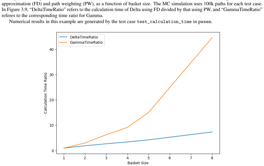
- For a basket of size $n$, raw path weighting computes the full Delta vector and Gamma matrix with $M$ paths, versus $2nM$ and $(2n^2+n)M$ paths for finite differences, and the raw estimator is unbiased.
- The adjusted Delta and Gamma estimators bring the variance from $O(\Delta t_1^{-1})$ and $O(\Delta t_1^{-2})$ down to $O(1)$ as the first time step shrinks, for payoffs with second-order generalised derivatives.
- For barrier-type payoffs with jumps, the adjusted Delta variance diverges only as $O(\Delta t_1^{-1/2})$ and adjusted Gamma as $O(\Delta t_1^{-3/2})$; first-order smoothing of payoff barriers reduces these rates further.
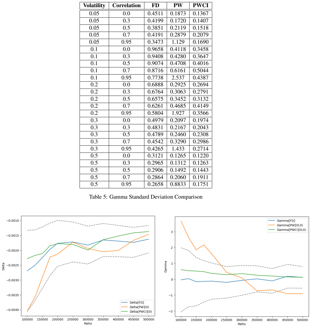
- Covariance inflation with the paper's suggested coefficients reduces Delta and Gamma standard deviation in near-singular cases such as correlation $0.95$ and low volatility, at the price of a bias claimed to be of order $O((\varepsilon_1+\varepsilon_2)\Delta t_1)$.
- In the reported numerical comparisons, adjusted path weighting matches or beats finite-difference standard deviation for Gamma in most settings and becomes competitive for Delta after covariance inflation.
Reading between the lines
- Because the weight formulas depend only on the first transition $H_0$, the method should combine unchanged with any discretisation scheme used after $t_1$, so it can be dropped into an existing Monte Carlo engine by modifying only the first step.
- The same reflection-and-zeroing variance reduction should carry over to other first-order sensitivities, such as vega or rho, by replacing $\partial_s H_0$ with the relevant parameter derivative, as long as the first-step map stays smooth and invertible.
- The variance-order results suggest a practical grid rule: place the deliberately small first step away from payoff event times, inserting an extra simulation point if necessary, so that the favourable $O(1)$ or fractional-divergence rates apply rather than the raw method's blow-up.
Editorial analysis
A structured set of objections, weighed in public.
Referee Report
Summary. The paper derives path weighting formulas for spot Delta and Gamma under a general functional discrete-time dynamics, proposes variance-reduced estimators for the case of a small first time step, and introduces a covariance inflation technique for singular or nearly singular covariance matrices. The main results are Theorem 2.2 (raw path weighting), Theorem 3.3 (variance-reduced adjustment), Theorem 3.8 and Lemma 3.13 (asymptotic variance orders), and Section 4 on covariance inflation. Numerical tests on autocallable payoffs and an open-source code library are included.
Significance. If the results are correct, the paper gives a practical way to compute the full Delta vector and Gamma matrix in one Monte Carlo simulation with controlled variance, which would be a substantial improvement over finite-difference Greeks for path-dependent derivatives. The Section 3 variance-reduction construction is an exact algebraic identity, and the variance-order theorems are proved and supported by numerical evidence. The covariance inflation part of Section 4, however, is the least supported component: its central bias bound is asserted rather than proved, and it appears to fail in the singular-correlation regime for which the section is designed. The paper's strengths are its explicit formulas, the inclusion of proofs for the core identities, reproducible open-source code, and numerical verification on industry-style autocallable payoffs.
major comments (3)
- [Section 4, Remark 4.4] The asserted bias bound C(ε1+ε2)Δt1 for covariance inflation is not a consequence of Theorem 4.1. Theorem 4.1 perturbs the noise argument inside a fixed map H1, while Definition 4.3 changes H1 itself by replacing σ0 and Σ with their inflated versions. In the correlated-diagonal form H1(s,x)=L(s,ρx), the parameter perturbation changes the column space of ρ; when Σ is singular, no mean-zero Y with exponential moments can satisfy L(s,√Δt1 ρε2 Z)=L(s,√Δt1 ρ(Z+εY)), because range(ρε2) is not contained in range(ρ). The claimed bound is in fact false in this regime: for two assets with ρ=1, equal volatilities, S0=(1,1), and payoff (S_T^(1)−S_T^(2))^+ (or a smooth approximation of it), the original price is zero, while the inflated process produces a first-step spread with variance of order ε2 σ² Δt1 and hence a price and Delta bias of order σ√(ε2 Δt1), not ε2 Δt1. Thus Remark 4.4 does not establish the reliability of covariance inflation in the singular case that Section 4 is intended to handle.
- [Section 4, Example 4.6, Tables 4 and 5] The numerical validation of PWCI reports only standard deviations of the estimators and never measures the bias introduced by covariance inflation against a reference value. Since the bias bound in Remark 4.4 is the load-bearing assertion for the method's practical reliability, tables showing variance reduction alone cannot establish that the total error stays within the discretization error. Please add bias or RMSE comparisons, especially for ρ close to 1 and for the singular case ρ=1, where the current analysis would predict bias of a larger order than the asserted bound.
- [Section 4, Theorem 4.1] The statement of Theorem 4.1 does not specify the regularity required of F; it calls F a payoff function without further assumptions. The proof, however, requires g(x)=E[F(St2,...,StN)|St1=H1(s,√Δt1,x)] to be C2, which is obtained by applying formula (2.9) to the conditional payoff. For a general measurable payoff with polynomial growth, this regularity is not automatic. The theorem should be stated with the needed smoothness assumption (or a separate approximation argument should be supplied) before it can be used as the basis for Remark 4.4.
minor comments (4)
- [Equation (2.12)] The notation 'δrp being the Dirac notation' should read 'Kronecker delta'; the symbol is used as a discrete index delta, not a Dirac delta.
- [Theorem 3.8, equation (3.17)] Equation (3.17) states Var(η1)=O(1) but the context and the definition of η2 show that the intended claim is Var(η2)=O(1) as Δt1→0.
- [Throughout] There are numerous typographical errors that should be corrected before publication, including 'the degenerator case' (Abstract and Section 4), 'addresses' used for 'address', 'Firgure' for 'Figure', 'estimagtors' for 'estimators', 'referes' for 'refers', 'crusial' for 'crucial', and 'finte' for 'finite'.
- [Section 4, Table 3] The inflation schedule ε2=0.5 e^{-10 λ̄} gives ε2=0.5 when λ̄=0, i.e., when the correlation is exactly singular; the paper should explicitly discuss this largest inflation case, since it is the extreme of the claimed bias-variance tradeoff.
Circularity Check
No significant circularity: the path weighting and variance-reduction results are derived self-containedly from the dynamics and Gaussian integration by parts, with no fitted parameters or load-bearing self-citations.
full rationale
The paper's central claims are derived in-line rather than imported from the authors' prior work. Theorem 2.2 is proved in Appendix 5.1 by differentiating the functional recursion and applying the standard Gaussian integration-by-parts lemma (Lemma 5.1); the Delta formula (2.6) and Gamma formula (2.9) follow directly from those manipulations with no fitted constants or assumed conclusion. The variance reduction adjustment in Theorem 3.3 is an exact algebraic rewriting using symmetry of the standard normal, and the proof exhibits the equalities (3.8)-(3.11) that make the adjusted estimators equal in expectation to the original ones. The asymptotic variance bounds in Theorem 3.8 and Lemma 3.13 are proved by bounding derivatives of the smoothed payoff, not by assuming the result. No load-bearing self-citation appears: the only reference is a standard textbook, and the numerical code repository is presented as implementation support rather than as justification of the mathematics. The covariance inflation parameters in Definition 4.3 are hand-chosen (epsilon_1 = 0.01, epsilon_2 = 0.5*exp(-10*lambda_bar)) and are not fitted to the target greeks, so the sensitivity estimates are not statistically forced. There is a genuine gap between Theorem 4.1, which covers noise perturbations of the form H1(s, sqrt(dt1)(Z1+epsilon Y)) with H1 fixed, and Remark 4.4, which applies the bound to parameter perturbations inside H1 itself; that is a correctness/rigor concern, not circularity, because the claimed bound is not obtained by definitionally reusing the target quantity. Overall the derivation chain is self-contained and non-circular.
Assumptions & free parameters
free parameters (2)
- epsilon1 (volatility inflation) =
0.01 in tests
- epsilon2 (correlation inflation schedule) =
0.5 * exp(-10 * lambda_bar) with lambda_bar = min |Lambda_kk|
assumptions (4)
- domain assumption The functional H0(s,x) is smooth in s and x, and the matrix ∂xH0 is invertible.
- domain assumption The functionals Hi have continuous second derivatives with at most polynomial growth, and ||J0(s,x)|| is bounded by a polynomial (Assumption 3.6).
- domain assumption For Theorem 4.1, the payoff F does not contain t1 as an event time and the perturbation Y has exponential moments.
- ad hoc to paper The covariance inflation bias bound extends from additive noise perturbations (Theorem 4.1) to parameter perturbations in Definition 4.3.
Cite this review
Pith. "Pith review of Path weighting sensitivities." pith.science (2026). https://pith.science/paper/TWW4XJVW
@misc{pith2026241113403,
  author       = {Pith},
  title        = {Pith review of: Path weighting sensitivities},
  year         = {2026},
  howpublished = {\url{https://pith.science/paper/TWW4XJVW}},
  note         = {Machine review of arXiv:2411.13403}
}
read the original abstract
In this paper, we study the computation of sensitivities with respect to spot of path dependent financial derivatives by means of path weighting. We propose explicit path weighting formula and variance reduction adjustment in order to address the large variance happening when the first simulation time step is small. We also propose a covariance inflation technique to addresses the degenerator case when the covariance matrix is singular. The stock dynamics we consider is given in a general functional form, which includes the classical Black-Scholes model, the implied distribution model, and the local volatility model.
Figures


Figures from the paper (10 more)



Reference graph
Works this paper leans on
-
[1]
[1] Glasserman, P. (2004). Monte Carlo Methods in Financial Engineering. 6Note that, for the conditional process, the ∆t1 in (2.9) becomes ∆t2 here. 25
work page 2004
Reviewed August 12, 2026 · model on record in the stance chip above.
Discussion (0). Continue with ORCID to comment.