REVIEW 2 major objections 6 minor 35 references
Implicit differentiation with second-order derivatives and benchmarks in finite-element-based differentiable physics
T0 review · 2 major / 6 minor · reviewed 2026-08-15 · deepseek-v4-flash
Pith's one-line read This paper derives a Hessian-vector product algorithm for implicit finite-element differentiation and shows that exact Hessians rescue Newton-CG where finite-difference Hessians diverge.
desk verdict A correct and useful Hessian-vector product primitive for implicit FEM, with benchmark claims that overreach because the finite-difference comparison is uncontrolled. read the letter →
The pith
A machine-rendered reading of the paper's core claim, the machinery that carries it, and where it could break.
The reading
What carries the argument
The load-bearing object is the bordered system of Eq. (15), formed from the Lagrangian $L(y,\lambda,\theta)=g(y,\theta)+\lambda^T r(y,\theta)$; its solution gives $\partial y/\partial\theta$ and $\partial\lambda/\partial\theta$. Algorithm 1 rewrites that system as two linear solves for the incremental state $\hat{y}$ and incremental adjoint $\hat{\lambda}$, then evaluates Eq. (22) to produce $H\hat{\theta}$. The essential mechanism is that second-order terms such as $(\partial/\partial\theta)(\lambda^T\partial r/\partial y)\hat{\theta}$ can be interpreted as nested Jacobian-vector and vector-Jacobian products, making the Hessian available solely from AD primitives rather than from hand-derived formulas.
What would settle it
Run the two benchmarks where Newton-CG (FD) diverges (source-field identification and traction identification) with a systematically tuned finite-difference step size, including central differences over a range of $h$ and gradient scaling. If a tuned finite-difference Hessian-vector product converges in comparable time, the paper's central contrast between exact and approximate Hessians collapses.
Extended reading notes
Core claim
The central claim is that the Hessian $d^2g/d\theta^2$ of an objective subject to an implicit finite-element constraint can be computed exactly, direction by direction, without forming the full matrix. The Hessian-vector product $H\hat{\theta}$ is assembled from four solves\textemdash forward state, adjoint, incremental forward, and incremental adjoint\textemdash combined in Eq. (22); each solve is linear even when the forward problem is nonlinear. All second-order terms in the assembly are compositions of Jacobian-vector and vector-Jacobian products, so a differentiable-programming library with those primitives can supply curvature automatically. The Taylor remainder test confirms that the residual of the second-order Taylor expansion decays as $\epsilon^3$, consistent with a machine-precision Hessian-vector product.
Load-bearing premise
The empirical conclusion that finite-difference Hessians are unusable rests on the assumption that the observed failures are inherent to finite differences rather than artifacts of an untuned step size; the derivation also assumes the bordered system matrix $\partial r/\partial y$ is nonsingular at every evaluation point.
Editorial extensions
If this is right
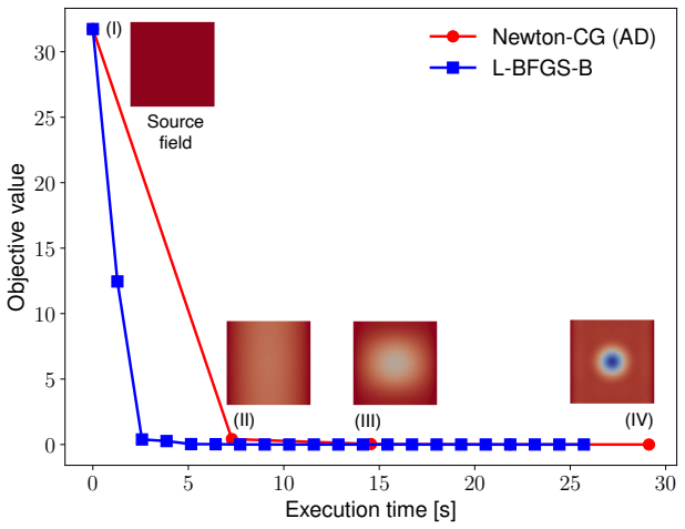
- On the nonlinear traction identification and shape-optimization benchmarks, Newton-CG with exact Hessian-vector products converges in wall-clock time faster than L-BFGS-B.
- On the linear source-identification and thermal-mechanical control benchmarks, L-BFGS-B converges faster, so the extra curvature is not always worth its cost.
- Finite-difference Hessian-vector products fail to converge in two of the four benchmarks, so exact implicit Hessians buy robustness, not just speed.
- Because the implicit Hessian approach solves each incremental problem once per direction and can cache the state and adjoint, repeated Hessian-vector products at a fixed parameter point are cheaper than repeated finite-difference gradient pairs.
Reading between the lines
- Beyond the paper: because the derivation only assumes an implicit residual equation, the same Hessian-vector product recipe transfers to non-finite-element implicit solvers.
- Beyond the paper: exact curvature enables Hessian-based uncertainty quantification, such as Laplace approximations of posterior covariances for PDE-constrained inverse problems.
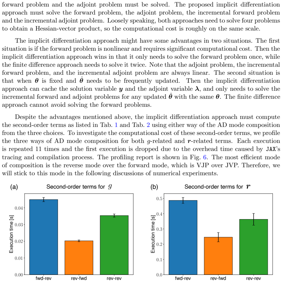
- Beyond the paper: the profiling results suggest that the choice of AD composition mode matters, and that exploiting sparsity in the second-order terms is a natural next step toward much larger problem sizes.
Signed reviews
Editorial analysis
A structured set of objections, weighed in public.
Referee Report
Summary. The manuscript derives an implicit Hessian-vector product for PDE-constrained optimization in a discretize-then-optimize framework, implements it in JAX-FEM using JVP/VJP primitives, and validates the implementation against finite-difference approximations and a Taylor remainder test. Four benchmark inverse problems are used to compare L-BFGS-B, Newton-CG with finite-difference Hessian-vector products (Newton-CG (FD)), and Newton-CG with the proposed implicit-differentiation Hessian-vector products (Newton-CG (AD)). The paper concludes that Newton-CG (AD) is robust and accelerates convergence for nonlinear problems, while L-BFGS-B is sufficient for linear problems, and that finite-difference Hessian approximations are unstable and inaccurate.
Significance. The core methodological contribution is sound and useful: the derivation in Section 2.3 is algebraically consistent, the algorithm in Section 3.1 is a natural and efficient composition of first-order implicit differentiation with JVP/VJP primitives, and the Taylor remainder test in Figure 5 provides independent, quantitative evidence that the Hessian-vector product is computed correctly to the expected third-order convergence. The public code is a strength, and the paper fills a real gap in differentiable FEM by making curvature information available as a primitive. The practical benchmark claims are only partially supported, however, because the comparison with finite-difference Hessians is not controlled and several benchmark settings are unreported. With those gaps fixed, the paper would make a solid contribution to the differentiable-physics community.
major comments (2)
- [Sections 4.1, 4.2, and 4.5] The claim that exact Hessians avoid "the instability and inaccuracy of finite difference Hessian approximations" is not established by the reported experiments, because Newton-CG (FD) is run with SciPy's default finite-difference Hessian-vector product and no step size, gradient tolerance, or other tuning is reported. The authors' own validation in Section 3.3.1 (Figures 3 and 4) shows that the finite-difference Hessian-vector product is strongly step-size dependent: the relative difference ranges from about 1e-3 at h=0.1 to about 1e-7 at h=1e-4. SciPy's default step for Newton-CG without a supplied Hessian is typically of order sqrt(machine epsilon) ~ 1.5e-8, which is two orders of magnitude smaller than the smallest h validated here and far below the usual optimum for a second-derivative estimate. The non-convergence of Newton-CG (FD) in Sections 4.1 and 4.2 may therefore be an artifact of the default step rather than of finite-difference Hessians in general. Please add a tuned-FD comparison, for example with h in the range 1e-4 to 1e-3 using Equation (28), and report all optimizer parameters; if tuned FD still fails to converge, the robustness claim is supported.
- [Section 4 (Eqs. (39), (43), (48), (49))] The benchmark protocol is under-specified and not fully reproducible: the regularization weights α introduced in Equations (39), (43), and (48) are never assigned numerical values, the optimizer tolerances, initial guesses, and linear solver settings are not reported, all convergence histories come from single runs, and the shape-optimization design mapping from the rotation angles to the density field in Section 4.4 is not defined. Consequently, the quantitative timing comparisons and the Section 4.5 recommendations ("Newton-CG faster for nonlinear, L-BFGS-B for linear") are not yet supported by the evidence as presented. Please report the complete settings for each benchmark and, where feasible, include multiple restarts or perturbation studies to show that the qualitative conclusions are robust.
minor comments (6)
- [Section 4 (multiple places)] The text repeatedly says "PDF-constrained optimization problem" where it should say "PDE-constrained optimization problem."
- [Figures 3 and 4] The x-axis tick labels are corrupted in the typeset version (for example, "0⊿000960" instead of a numeric value with a power-of-ten notation); the figures should be regenerated with proper mathematical notation.
- [Section 3.3.1] The step-size sweep stops at h=10^-4; adding values near the expected optimum for a second-derivative estimate, roughly h ~ eps^(1/3), would make the accuracy validation more convincing.
- [Section 2.3, Eq. (15)] The derivation implicitly assumes that the bordered KKT matrix, in particular ∂r/∂y, is nonsingular at every evaluation point; this implicit-function-theorem hypothesis should be stated explicitly as an assumption on the admissible parameter set.
- [Section 4.4] The mapping from the rotation angles θ to the density field ρ(x) through the sigmoid function is not defined; for reproducibility, the manuscript should give the exact formula and any smoothing or length-scale parameters.
- [Algorithm 1] Steps 1 and 2 require solving a nonlinear forward problem and a linear adjoint problem, respectively; the intended numerical solver and convergence criterion for these solves should be specified.
Circularity Check
No circularity found: the implicit Hessian-vector product is derived from the residual and objective via the Lagrangian, and the Taylor remainder test independently validates it against objective evaluations.
full rationale
The paper's central object, the implicit Hessian-vector product Hθhat, is derived in Section 2.3 by differentiating the first-order optimality conditions of the Lagrangian (Eqs. (15)-(22)); this is a self-contained derivation from the residual r(y,theta)=0 and objective g(y,theta), not an input fitted to the outputs it claims to predict. The implementation in Algorithm 1 composes JAX JVP/VJP primitives to evaluate those derived terms, and accuracy is checked two ways: against central finite differences of the derived gradient (Eq. (28)) and, independently, against the third-order Taylor remainder (Eq. (36), Fig. 5). Neither check reuses the Hessian formula as its own evidence: the Taylor test compares the computed gradient and Hessian against direct objective evaluations, and the FD comparison uses a different computation path. The only self-citation to JAX-FEM [13] supplies the first-order gradient baseline and FEM infrastructure, but the gradient is also derived in Eqs. (12)-(14), and the Hessian derivation does not assume the truth of that citation. The benchmarking claim that Newton-CG (FD) is unreliable because SciPy's default FD Hessian failed in two examples is an experimental-control concern, not circularity, since the comparison is not constructed from fitted values or definitions that guarantee the conclusion. No self-definitional, fitted-input, or citation-imported uniqueness step was found.
Assumptions & free parameters
free parameters (1)
- Regularization weight α in benchmarks =
Not reported
assumptions (3)
- domain assumption The discrete residual r(y,θ)=0 implicitly defines y(θ) and the bordered KKT matrix in Eq. (15) is nonsingular (in particular ∂r/∂y is invertible).
- standard math The Lagrangian L is C² so mixed partials commute, as used to equate the transposed block vector in Eq. (19).
- domain assumption JAX's JVP and VJP primitives compute exact derivatives of the assembled finite element residual and objective.
Cite this review
Pith. "Pith review of Implicit differentiation with second-order derivatives and benchmarks in finite-element-based differentiable physics." pith.science (2026). https://pith.science/paper/U2C7UPJX
@misc{pith2026250512646,
  author       = {Pith},
  title        = {Pith review of: Implicit differentiation with second-order derivatives and benchmarks in finite-element-based differentiable physics},
  year         = {2026},
  howpublished = {\url{https://pith.science/paper/U2C7UPJX}},
  note         = {Machine review of arXiv:2505.12646}
}
read the original abstract
Differentiable programming is revolutionizing computational science by enabling automatic differentiation (AD) of numerical simulations. While first-order gradients are well-established, second-order derivatives (Hessians) for implicit functions in finite-element-based differentiable physics remain underexplored. This work bridges this gap by deriving and implementing a framework for implicit Hessian computation in PDE-constrained optimization problems. We leverage primitive AD tools (Jacobian-vector product/vector-Jacobian product) to build an algorithm for Hessian-vector products and validate the accuracy against finite difference approximations. Four benchmarks spanning linear/nonlinear, 2D/3D, and single/coupled-variable problems demonstrate the utility of second-order information. Results show that the Newton-CG method with exact Hessians accelerates convergence for nonlinear inverse problems (e.g., traction force identification, shape optimization), while the L-BFGS-B method suffices for linear cases. Our work provides a robust foundation for integrating second-order implicit differentiation into differentiable physics engines, enabling faster and more reliable optimization.
Figures


Figures from the paper (14 more)





Reference graph
Works this paper leans on
-
[1]
The elements of differentiable programming
Mathieu Blondel and Vincent Roulet. The elements of differentiable programming. arXiv preprint arXiv:2403.14606, 2024
arXiv 2024
-
[2]
Deep learning
Yann LeCun, Yoshua Bengio, and Geoffrey Hinton. Deep learning. nature, 521(7553):436–444, 2015
2015
-
[3]
Jax: composable transformations of python+ numpy programs
James Bradbury, Roy Frostig, Peter Hawkins, Matthew James Johnson, Chris Leary, Dougal Maclaurin, George Necula, Adam Paszke, Jake VanderPlas, Skye Wanderman-Milne, et al. Jax: composable transformations of python+ numpy programs. 2018
2018
-
[4]
Pytorch: An imperative style, high-performance deep learning library
A Paszke. Pytorch: An imperative style, high-performance deep learning library. arXiv preprint arXiv:1912.01703, 2019
arXiv 1912
-
[5]
Jax-fluids: A fully-differentiable high-order computational fluid dynamics solver for compressible two-phase flows
Deniz A Bezgin, Aaron B Buhendwa, and Nikolaus A Adams. Jax-fluids: A fully-differentiable high-order computational fluid dynamics solver for compressible two-phase flows. Computer Physics Communications, 282:108527, 2023
2023
-
[6]
Machine learning–accelerated computational fluid dynamics.Proceedings of the National Academy of Sciences, 118(21):e2101784118, 2021
Dmitrii Kochkov, Jamie A Smith, Ayya Alieva, Qing Wang, Michael P Brenner, and Stephan Hoyer. Machine learning–accelerated computational fluid dynamics.Proceedings of the National Academy of Sciences, 118(21):e2101784118, 2021
2021
-
[7]
Jax md: a framework for differentiable physics
Samuel Schoenholz and Ekin Dogus Cubuk. Jax md: a framework for differentiable physics. Advances in Neural Information Processing Systems , 33, 2020
work page 2020
-
[8]
Simplifying fft-based methods for solid mechanics with au- tomatic differentiation
Mohit Pundir and David S Kammer. Simplifying fft-based methods for solid mechanics with au- tomatic differentiation. Computer Methods in Applied Mechanics and Engineering, 435:117572, 2025
work page 2025
Show all 35 references
-
[9]
Neural-integrated meshfree (nim) method: A differentiable programming-based hybrid solver for computational mechanics
Honghui Du and QiZhi He. Neural-integrated meshfree (nim) method: A differentiable programming-based hybrid solver for computational mechanics. Computer Methods in Applied Mechanics and Engineering, 427:117024, 2024
2024
-
[10]
Jax-bte: a gpu-accelerated differentiable solver for phonon boltzmann transport equations
Wenjie Shang, Jiahang Zhou, JP Panda, Zhihao Xu, Yi Liu, Pan Du, Jian-Xun Wang, and Tengfei Luo. Jax-bte: a gpu-accelerated differentiable solver for phonon boltzmann transport equations. npj Computational Materials , 11(1):1–12, 2025. 28
2025
-
[11]
Adjoint sensitivity analysis for differential-algebraic equations: The adjoint DAE system and its numerical solution
Yang Cao, Shengtai Li, Linda Petzold, and Radu Serban. Adjoint sensitivity analysis for differential-algebraic equations: The adjoint DAE system and its numerical solution. SIAM Journal on Scientific Computing , 24(3):1076–1089, 2003
2003
-
[12]
Efficient and modular implicit differentia- tion
Mathieu Blondel, Quentin Berthet, Marco Cuturi, Roy Frostig, Stephan Hoyer, Felipe Llinares- L´ opez, Fabian Pedregosa, and Jean-Philippe Vert. Efficient and modular implicit differentia- tion. Advances in neural information processing systems , 35:5230–5242, 2022
2022
-
[13]
Jax-fem: A differentiable gpu-accelerated 3d finite element solver for automatic inverse design and mechanistic data science
Tianju Xue, Shuheng Liao, Zhengtao Gan, Chanwook Park, Xiaoyu Xie, Wing Kam Liu, and Jian Cao. Jax-fem: A differentiable gpu-accelerated 3d finite element solver for automatic inverse design and mechanistic data science. Computer Physics Communications , 291:108802, 2023
2023
-
[14]
The finite element method: linear static and dynamic finite element analysis
Thomas JR Hughes. The finite element method: linear static and dynamic finite element analysis. Courier Corporation, 2003
2003
-
[15]
springer, 2019
Joel H Ferziger, Milovan Peri´ c, and Robert L Street.Computational methods for fluid dynamics. springer, 2019
2019
-
[16]
Meshfree methods: moving beyond the finite element method
Gui-Rong Liu. Meshfree methods: moving beyond the finite element method . CRC press, 2009
2009
-
[17]
Optimal solvers for pde-constrained optimization
Tyrone Rees, H Sue Dollar, and Andrew J Wathen. Optimal solvers for pde-constrained optimization. SIAM Journal on Scientific Computing , 32(1):271–298, 2010
2010
-
[18]
Function minimization by conjugate gradients
Reeves Fletcher and Colin M Reeves. Function minimization by conjugate gradients. The computer journal, 7(2):149–154, 1964
1964
-
[19]
Newton-type minimization via the lanczos method
Stephen G Nash. Newton-type minimization via the lanczos method. SIAM Journal on Nu- merical Analysis, 21(4):770–788, 1984
1984
-
[20]
A reduced hessian method for large-scale constrained optimization
Lorenz T Biegler, Jorge Nocedal, and Claudia Schmid. A reduced hessian method for large-scale constrained optimization. SIAM Journal on Optimization , 5(2):314–347, 1995
1995
-
[21]
Numerical optimization
Jorge Nocedal and Stephen J Wright. Numerical optimization. Springer, 1999
1999
-
[22]
Fractional pde constrained optimization: An optimize- then-discretize approach with l-bfgs and approximate inverse preconditioning
Stefano Cipolla and Fabio Durastante. Fractional pde constrained optimization: An optimize- then-discretize approach with l-bfgs and approximate inverse preconditioning. Applied Numer- ical Mathematics, 123:43–57, 2018
2018
-
[23]
Discretize then optimize
John T Betts and Stephen L Campbell. Discretize then optimize. Mathematics for industry: challenges and frontiers , pages 140–157, 2005
2005
-
[24]
A computational framework for infinite-dimensional bayesian inverse problems part i: The linearized case, with application to global seismic inversion
Tan Bui-Thanh, Omar Ghattas, James Martin, and Georg Stadler. A computational framework for infinite-dimensional bayesian inverse problems part i: The linearized case, with application to global seismic inversion. SIAM Journal on Scientific Computing , 35(6):A2494–A2523, 2013
2013
-
[25]
hippylib: An extensible software framework for large-scale inverse problems governed by pdes: Part i: Deterministic inversion and linearized bayesian inference
Umberto Villa, Noemi Petra, and Omar Ghattas. hippylib: An extensible software framework for large-scale inverse problems governed by pdes: Part i: Deterministic inversion and linearized bayesian inference. ACM Transactions on Mathematical Software (TOMS) , 47(2):1–34, 2021
2021
-
[26]
dolfin-adjoint 2018.1: automated ad- joints for fenics and firedrake
Sebastian Mitusch, Simon Funke, and Jørgen Dokken. dolfin-adjoint 2018.1: automated ad- joints for fenics and firedrake. Journal of Open Source Software , 4(38):1292, 2019
2018
-
[27]
Adjoint optimization of pressurized membrane structures using automatic differentiation tools
Alexander Niewiarowski, Sigrid Adriaenssens, and Ruy Marcelo Pauletti. Adjoint optimization of pressurized membrane structures using automatic differentiation tools. Computer Methods in applied mechanics and engineering , 372:113393, 2020. 29
2020
-
[28]
Mapped shape optimization method for the rational design of cellular mechanical metamaterials under large deformation
Tianju Xue and Sheng Mao. Mapped shape optimization method for the rational design of cellular mechanical metamaterials under large deformation. International journal for numerical methods in engineering, 123(10):2357–2380, 2022
2022
-
[29]
Principles of mathematical analysis
Walter Rudin. Principles of mathematical analysis . McGraw-Hill Book Company, Inc., New York-Toronto-London, 1953
1953
-
[30]
Sparser, better, faster, stronger: Efficient automatic differ- entiation for sparse jacobians and hessians
Adrian Hill and Guillaume Dalle. Sparser, better, faster, stronger: Efficient automatic differ- entiation for sparse jacobians and hessians. arXiv preprint arXiv:2501.17737 , 2025
2025 arXiv
-
[31]
Algorithm 778: L-bfgs-b: Fortran subroutines for large-scale bound-constrained optimization
Ciyou Zhu, Richard H Byrd, Peihuang Lu, and Jorge Nocedal. Algorithm 778: L-bfgs-b: Fortran subroutines for large-scale bound-constrained optimization. ACM Transactions on mathematical software (TOMS), 23(4):550–560, 1997
1997
-
[32]
Scipy 1.0: fundamental algorithms for scientific computing in python.Nature methods, 17(3):261–272, 2020
Pauli Virtanen, Ralf Gommers, Travis E Oliphant, Matt Haberland, Tyler Reddy, David Cour- napeau, Evgeni Burovski, Pearu Peterson, Warren Weckesser, Jonathan Bright, et al. Scipy 1.0: fundamental algorithms for scientific computing in python.Nature methods, 17(3):261–272, 2020
2020
-
[33]
Non-contact reconstitution of the traction distribution using in- complete deformation measurements: Methodology and experimental validation
Yue Mei, Dongmei Zhao, Rongyao Kang, Xinyu Wang, Bo Wang, Dawei Song, Li Dong, Hao Jiang, and Stephane Avril. Non-contact reconstitution of the traction distribution using in- complete deformation measurements: Methodology and experimental validation. International Journal of ...
2024
-
[34]
Non-linear elastic deformations
Raymond W Ogden. Non-linear elastic deformations . Courier Corporation, 1997
1997
-
[35]
Topology optimization: theory, methods, and appli- cations
Martin Philip Bendsoe and Ole Sigmund. Topology optimization: theory, methods, and appli- cations. Springer Science & Business Media, 2013. 30
2013
Reviewed August 15, 2026 · model on record in the stance chip above.
Discussion (0). Continue with ORCID to comment.