REVIEW 3 major objections 4 minor 37 references
ResiPhy-MDNF: A Residual-Based Physics-Aware Multilevel Discrete Neural Field Framework for PDE-Constrained Inverse Problems
T0 review · 3 major / 4 minor · reviewed 2026-08-02 · deepseek-v4-flash
Pith's one-line read A learned coarse-to-fine transfer over nested discrete neural fields recovers PDE coefficients more accurately than optimizing directly on the finest grid, at modest extra grid work.
desk verdict Genuinely new per-instance learned transfer for multilevel inverse problems with a credible matched ablation—but the headline cost number omits corrector fitting, so the efficiency claim is overstated. read the letter →
The pith
A machine-rendered reading of the paper's core claim, the machinery that carries it, and where it could break.
The reading
What carries the argument
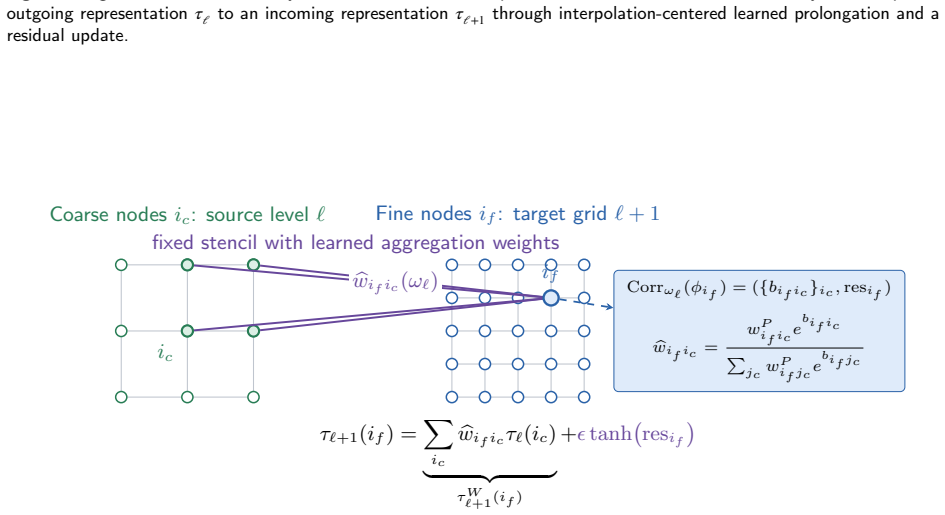
The load-bearing component is ResiPhy-GNN, a graph neural network performing learned coarse-to-fine prolongation. Each fine node aggregates from a fixed coarse stencil using an interpolation-centered softmax: the prescribed bilinear weights are multiplied by learned edge-logit exponentials and renormalized, so the all-zero case recovers bilinear interpolation exactly. The aggregated value is then updated by a bounded correction (epsilon times tanh of a residual). A shared two-layer SiLU MLP, applied pointwise to node features (coordinates, interpolated baseline, observation and source channels, and an optional loss-gradient diagnostic), outputs the logit biases and the residual; the output l
What would settle it
Run the direct 128 Darcy solve with enough extra Adam steps to match the multilevel path's total Adam-step budget (about 10,500 steps at the fine-grid-equivalent cost, including the 3,000 transfer steps). If its error drops to the multilevel level, the claimed advantage is a compute-budget effect rather than a property of the coarse-to-fine path.
Extended reading notes
Core claim
The central claim is that a per-instance, objective-fitted graph-network transfer (ResiPhy-GNN) over nested discrete neural field levels yields better reconstructions than direct single-level DNF optimization at similar cost. The transfer starts from bilinear interpolation, then learns edge-logit biases and a bounded nodewise correction by minimizing the target-level physics and data loss. In a controlled Darcy test, the 64-to-128 path uses 1.25x the cumulative grid-work proxy of the direct 128 solve while achieving 6.76x lower permeability error and 10.4x lower state error. On measured EIT data, the same construction improves the mean thresholded three-class overlap from 0.603 to 0.623. No
Load-bearing premise
The reported 1.25x cost factor counts only the DNF solver steps on each grid and omits the 3000 Adam steps spent fitting the GNN transfer at each interface; if the transfer cost is included, the true overhead is roughly 1.75x for the one-interface Darcy path (and larger for three-interface runs), so the strength of the 'similar cost' claim depends on this accounting.
Editorial extensions
If this is right
- The error reductions persist over the full fine-grid optimization trajectory in the matched reservoir-like Darcy ablation, so the learned transfer improves the optimization path itself, not just the starting point.
- The same multilevel construction works for both full-space Darcy inversion and reduced linearized EIT inversion, indicating the transfer module is not tied to a specific PDE, discretization, or observation geometry.
- Because the transfer is fitted per instance using the prescribed numerical operator, the framework inherits the physics model directly and avoids the risk of surrogate errors being absorbed into the reconstructed coefficient.
- The complete four-level run shows the approach scales to three interfaces while reducing the normalized PDE residual at each transition, with the largest reduction at the final coarse-to-fine step.
Reading between the lines
- Including the 3000 Adam transfer-fitting steps (assessed at the target grid) in the cost accounting would raise the reported 1.25x work proxy to roughly 1.75x for one interface and more for three; the efficiency-precision trade-off likely remains favorable, but a full wall-clock comparison would settle it.
- The per-instance fitting makes the method expensive when many levels are stacked; warm-starting or sharing corrector parameters across similar problems could cut that overhead, at the cost of the paper's deliberate no-pretraining design.
- The residual update is bounded and the weights are interpolation-centered, suggesting the learned correction acts as a form of instance-adaptive regularization; one could test whether it degrades gracefully as observation noise increases, since the transfer loss includes the noisy data.
- The graph-based formulation does not assume Cartesian structure, so the framework may extend to unstructured and adaptively refined meshes; the paper explicitly leaves this as future work, and a test on a triangular-mesh Darcy or EIT problem would be a natural check.
Signed reviews
Editorial analysis
A structured set of objections, weighed in public.
Referee Report
Summary. The paper introduces ResiPhy-MDNF, a multilevel framework for PDE-constrained coefficient inverse problems. On each resolution level, a Discrete Neural Field (DNF) optimizer directly updates discrete state and coefficient arrays under the prescribed numerical model, without surrogate models or offline training. Between levels, a per-instance graph neural network, ResiPhy-GNN, is fitted to the target-level transfer loss and produces a corrected coarse-to-fine initialization. The method is instantiated for full-space Darcy permeability inversion and for reduced linearized complete-electrode-model EIT on the KTC2023 dataset. The main reported results are: a controlled Darcy comparison in which the 64^2→128^2 path uses 1.25× the cumulative grid-work proxy of the direct 128^2 solve while reducing coefficient and state errors by factors of 6.76 and 10.4; a matched LUNDIsim ablation in which ResiPhy-GNN transfer improves final errors by about 8–9% over simple interpolation; and a KTC2023 EIT pipeline that reaches 0.623 mean mIoU versus 0.603 for the official linearized CEM reconstruction and 0.533 for direct single-level DNF. The paper argues that the same multilevel construction transfers across different PDEs, discretizations, and observation geometries.
Significance. If the results hold, the framework is a practical and interesting contribution: it retains the prescribed numerical operator, requires no offline training, and shows that a per-instance learned transfer can improve coarse-to-fine inverse optimization. The matched LUNDIsim ablation in Section 5.3 is a genuine strength: it isolates the transfer mechanism from the multilevel path and shows a consistent improvement under identical fine-grid optimization budgets. The per-instance fitting of the transfer also avoids the circularity risk that would come from using fine-grid truth during transfer training. The main quantitative claim, however, is the efficiency-precision trade-off in the Darcy experiment, and that claim rests on a cost proxy that omits a substantial part of the actual computation. The qualitative conclusion may survive correction, but the headline numbers and the wording need revision. The KTC2023 comparison is less controlled than the Darcy/LUNDIsim comparisons and should be presented with appropriate caveats or supplemented with a matched baseline.
major comments (3)
- [§5.2, Eq. (38); §5.1; Abstract] The headline '1.25× cumulative grid-work proxy' omits the cost of fitting ResiPhy-GNN. Section 5.1 states that correctors are fitted for 3000 Adam steps, and the Darcy transfer loss (29) is evaluated on the refined target grid. Equation (38), however, counts only the DNF-level steps s_k=6000 at each grid. For the 64^2→128^2 basic case, the reported numerator is 6000·64^2 + 6000·128^2, giving 1.25× the direct 128^2 cost. Adding the 3000 transfer-fitting Adam steps at 128^2 gives 6000·64^2 + 6000·128^2 + 3000·128^2, which is about 1.75× the direct cost, not 1.25×. For the four-level LUNDIsim run, three transfer fittings are omitted, so the undercount is larger. The manuscript is internally consistent about what Eq. (38) counts, but Section 5.2 calls this a 'quantified total-work comparison,' and the abstract presents 1.25× without qualification. This is load-bearing for the 'similar cost'
- [§5.5, Table 5] The KTC2023 comparison between single-level DNF and ResiPhy-MDNF is not matched. The single-level baseline uses 10,000 Adam updates with the official-setting regularization, while the complete pipeline uses 1200 coarse-grid Adam updates, eight corrector L-BFGS iterations, and 60 outer mesh-L-BFGS updates, together with the full measurement matrix and the adaptively chosen conductivity weight (34). The text acknowledges that 'an Adam and an L-BFGS update differ in cost,' but the table and the introduction still present the mIoU gain as evidence in favor of the complete pipeline. Because the optimizer, loss weighting, and computational budget all differ, this comparison does not isolate the multilevel/DNF effect. The matched LUNDIsim ablation is the correct evidence for the transfer, and the KTC2023 section should be framed as a full-pipeline comparison only. If the cross-physics claim is
- [§2.2, §3.3, Table 3] The claim that the framework is 'the same multilevel construction' across Darcy and EIT is somewhat overstated because the EIT realization has only one transfer interface and two DNF stages, and it uses a linearized reduced-space model rather than the full-space DNF formulation used for Darcy. This is not an error, but the paper's framing in the abstract and introduction suggests a more uniform hierarchy than is actually instantiated. The transfer-loss and feature constructions are analogous, and the matched LUNDIsim experiment provides the controlled evidence, so this is a presentation issue rather than a technical flaw. I recommend that the cross-physics claim be stated as 'the same transfer module can be instantiated for two different linear/full-space formulations,' which is well supported.
minor comments (4)
- [§5.1, §5.2] The 'relative L2 errors' E_K and E_U used in Table 2 and Eq. (39) are not formally defined. Please state whether these are normalized by the L2 norm of the reference field and over which grid points or cells they are computed.
- [§5.3, Figure 4] The transfer ablation in Table 3 is reported for a single LUNDIsim instance without multiple random seeds or repeated runs. The reported improvements of about 8–9% are modest; please state whether the optimizations are deterministic and, if not, report mean and variance over seeds.
- [§4.2, Eq. (34)] The measurement-energy rule for lambda_sigma is calibrated once from Data 1 and then applied to all phantoms. The paper states this clearly, but please make explicit in the text that the calibration does not see the reconstructions and is not tuned per phantom, so that the reader does not confuse this with an oracle choice.
- [Throughout] There are numerous missing spaces in the abstract and main text around math and words (e.g., '642 →128 2', 'medium' appears as 'medum', etc.). These appear to be PDF-extraction artifacts, but the final journal version should have a clean text layer.
Circularity Check
No circular derivation: the transfer is fitted to the target-level objective, and all reported errors are evaluated against ground truth; the cost-proxy caveat is an accounting issue, not circularity.
full rationale
The paper's derivation chain is self-contained with respect to circularity. The DNF loss in Eq. (13) is the optimization objective; the ResiPhy-GNN transfer minimizes the fixed transfer loss in Eqs. (20)/(29), which couples only the target-grid PDE residual and observed pressures, with no fine-grid reference fields. The subsequent DNF solve in Eq. (21) continues optimizing the same reconstruction objective from the transferred initialization, and Tables 2 and 3 report errors against held-out ground-truth fields. No reported metric is defined by the fitted transfer parameters. The c_S calibration in Eq. (34) uses Data 1 voltage energy only to set the regularization weight lambda_sigma, not the reported mIoU, and the paper explicitly states that no reconstruction or segmentation labels enter that calibration. References to ODIL, PIXEL, and GNN message passing are external prior work, not load-bearing self-citations, and no uniqueness theorem is imported from the authors' own prior results. The one notable weakness is efficiency accounting: Eq. (38) counts DNF Adam steps but omits the 3000-step per-interface ResiPhy-GNN fitting described in Section 5.1, so the '1.25x' grid-work proxy understates full computational cost (about 1.75x for a single transfer). This is an incomplete cost metric, not a self-referential or definitional reduction, and it does not make the reported error reductions circular.
Assumptions & free parameters
free parameters (4)
- c_S (measurement-energy rule constant) =
8.7228432763e-6
- λ_σ values for EIT =
(0.3000, 0.1464, 0.1023, 0.04195)
- Darcy loss weights λ_pde, λ_obs, λ_K and coefficient-freeze schedule =
not specified
- Transfer/correction hyperparameters =
ε_u=ε_ρ=0.1, w_pde=1, w_obs=1000, 3000 Adam steps, L-BFGS iterations, η=0.3
assumptions (4)
- standard math The conservative finite-difference residual (8) with harmonic transmissibility is a consistent discretization of the Darcy equation (7).
- domain assumption The linearized complete electrode model (11) adequately represents KTC2023 difference imaging.
- domain assumption The transfer can be fitted from the target-level objective alone, without fine-grid truth, to produce beneficial initializations.
- domain assumption Otsu thresholding of the continuous reconstructions is an appropriate evaluation for the EIT task.
Cite this review
Pith. "Pith review of ResiPhy-MDNF: A Residual-Based Physics-Aware Multilevel Discrete Neural Field Framework for PDE-Constrained Inverse Problems." pith.science (2026). https://pith.science/paper/U2QBNTD2
@misc{pith2026260706237,
  author       = {Pith},
  title        = {Pith review of: ResiPhy-MDNF: A Residual-Based Physics-Aware Multilevel Discrete Neural Field Framework for PDE-Constrained Inverse Problems},
  year         = {2026},
  howpublished = {\url{https://pith.science/paper/U2QBNTD2}},
  note         = {Machine review of arXiv:2607.06237}
}
abstract
Inverse problems governed by partial differential equations are difficult when observations are sparse and the unknown coefficient field contains both large- and small-scale structures. We introduce a residual-based, physics-aware multilevel discrete neural field framework, ResiPhy-MDNF, for such problems. The method couples a coarse-to-fine discrete neural field (DNF) optimizer with a residual-based graph neural network (GNN) transfer operator, called ResiPhy-GNN. At each level, the DNF directly optimizes trainable grid- or mesh-based state and coefficient arrays using the prescribed numerical model. Between levels, ResiPhy-GNN maps the coarse representation to the fine representation through a learned prolongation based on graph connectivity, spatial features, and residual information. The method requires neither surrogate models nor offline pretraining. We evaluate the framework on coefficient inversion in Darcy flow for subsurface modeling and on electrical impedance tomography (EIT). In the controlled Darcy test case, the \(64^2\!\to128^2\) multilevel path uses \(1.25\times\) the cumulative grid-work proxy of the direct single-level \(128^2\) solve, while achieving \(6.76\times\) lower permeability error and \(10.4\times\) lower state error. On measured Kuopio Tomography Challenge 2023 EIT data, the framework improves the mean intersection-over-union after Otsu thresholding by roughly \(3.4\%\) over the official linearized complete electrode model reconstruction and by \(16.9\%\) over direct single-level discrete-field optimization. These results indicate that the same multilevel construction can be used across different coefficient structures, discretizations, and observation geometries.
Figures


Figures from the paper (11 more)


Reference graph
Works this paper leans on
-
[1]
Alghamdi,A.M.A.,Carøe,M.S.,Everink,J.M.,Jørgensen,J.S.,Knudsen,K.,Nielsen,J.T.K.,Rasmussen,A.K.,Sørensen,R.K.H.,Zhang,C.,
-
[2]
A multigrid method for distributed parameter estimation problems
Ascher, U.M., Haber, E., 2003. A multigrid method for distributed parameter estimation problems. Electronic Transactions on Numerical Analysis 15, 1–17. URL:https://etna.ricam.oeaw.ac.at/volumes/2001-2010/vol15/
2003
-
[3]
The cascadic multigrid method for elliptic problems
Bornemann, F.A., Deuflhard, P., 1996. The cascadic multigrid method for elliptic problems. Numerische Mathematik 75, 135–152. doi:10.1007/s002110050234
-
[4]
Computational Optimization of Systems Governed by Partial Differential Equations
Borzì, A., Schulz, V., 2012. Computational Optimization of Systems Governed by Partial Differential Equations. volume 8 ofComputational Science & Engineering. SIAM, Philadelphia. doi:10.1137/1.9781611972054
-
[5]
Multigrid methods for PDE optimization
Borzì, A., Schulz, V.H., 2009. Multigrid methods for PDE optimization. SIAM Review 51, 361–395. doi:10.1137/060671590
-
[6]
Brandt,A.,Livne,O.E.,2011. Fullmulti-grid(FMG)algorithms,in:MultigridTechniques:1984GuidewithApplicationstoFluidDynamics, Revised Edition. Society for Industrial and Applied Mathematics, Philadelphia. volume 67 ofClassics in Applied Mathematics, pp. 75–81. doi:10.1137/1.9781611970753.ch7
-
[7]
Multibang regularization for electrical impedance tomography
Brandt, C., Do, T.B.T., Horn, P., 2024. Multibang regularization for electrical impedance tomography. Applied Mathematics for Modern Challenges 2, 208–227. doi:10.3934/ammc.2024007
-
[8]
Lundisim: Model meshes for flow simulation and scientific data compression benchmarks
Duval, L., Payan, F., Preux, C., Bouard, L., 2025. Lundisim: Model meshes for flow simulation and scientific data compression benchmarks. Geoscience Data Journal 12, e70030. URL:https://rmets.onlinelibrary.wiley.com/doi/10.1002/gdj3.70030, doi:10.1002/ gdj3.70030
Show all 37 references
-
[9]
Neuralmessagepassingforquantumchemistry,in:Proceedingsofthe 34thInternationalConferenceonMachineLearning,PMLR.pp.1263–1272.URL:https://proceedings.mlr.press/v70/gilmer17a
Gilmer,J.,Schoenholz,S.S.,Riley,P.F.,Vinyals,O.,Dahl,G.E.,2017. Neuralmessagepassingforquantumchemistry,in:Proceedingsofthe 34thInternationalConferenceonMachineLearning,PMLR.pp.1263–1272.URL:https://proceedings.mlr.press/v70/gilmer17a. html
2017
-
[10]
Optimization with PDE Constraints
Hinze, M., Pinnau, R., Ulbrich, M., Ulbrich, S., 2009. Optimization with PDE Constraints. volume 23 ofMathematical Modelling: Theory and Applications. Springer, Dordrecht. doi:10.1007/978-1-4020-8839-1
2009 doi
-
[11]
Statistical and Computational Inverse Problems
Kaipio, J., Somersalo, E., 2005. Statistical and Computational Inverse Problems. volume 160 ofApplied Mathematical Sciences. Springer, New York. doi:10.1007/b138659
2005 doi
-
[12]
PIXEL: Physics-informed cell representations for fast and accurate PDE solvers, in: Proceedings of the AAAI Conference on Artificial Intelligence, pp
Kang, N., Lee, B., Hong, Y., Yun, S.B., Park, E., 2023. PIXEL: Physics-informed cell representations for fast and accurate PDE solvers, in: Proceedings of the AAAI Conference on Artificial Intelligence, pp. 8186–8194. doi:10.1609/aaai.v37i7.25988,arXiv:2207.12800
2023 arXiv
-
[13]
Solving inverse problems in physics by optimizing a discrete loss: Fast and accurate learning without neural networks
Karnakov, P., Litvinov, S., Koumoutsakos, P., 2024. Solving inverse problems in physics by optimizing a discrete loss: Fast and accurate learning without neural networks. PNAS Nexus 3, pgae005. doi:10.1093/pnasnexus/pgae005
2024 doi
-
[14]
Physics-informed machine learning
Karniadakis, G.E., Kevrekidis, I.G., Lu, L., Perdikaris, P., Wang, S., Yang, L., 2021. Physics-informed machine learning. Nature Reviews Physics 3, 422–440. doi:10.1038/s42254-021-00314-5
2021 doi
- [15]
-
[16]
URL:https://openreview.net/forum?id=c8P9NQVtmnO,arXiv:2010.08895.internationalConference on Learning Representations
Li,Z.,Kovachki,N.B.,Azizzadenesheli,K.,Liu,B.,Bhattacharya,K.,Stuart,A.,Anandkumar,A.,2021.Fourierneuraloperatorforparametric partialdifferentialequations. URL:https://openreview.net/forum?id=c8P9NQVtmnO,arXiv:2010.08895.internationalConference on Learning Representations
2021 arXiv
-
[17]
Optimal Control of Systems Governed by Partial Differential Equations
Lions, J.L., 1971. Optimal Control of Systems Governed by Partial Differential Equations. volume 170 ofGrundlehren der mathematischen Wissenschaften. Springer, Berlin, Heidelberg. doi:10.1007/978-3-642-65024-6
1971 doi
-
[18]
On the limited memory BFGS method for large scale optimization
Liu, D.C., Nocedal, J., 1989. On the limited memory BFGS method for large scale optimization. Mathematical Programming 45, 503–528. doi:10.1007/BF01589116
1989 doi
-
[19]
LearningnonlinearoperatorsviaDeepONetbasedontheuniversalapproximation theorem of operators
Lu,L.,Jin,P.,Pang,G.,Zhang,Z.,Karniadakis,G.E.,2021. LearningnonlinearoperatorsviaDeepONetbasedontheuniversalapproximation theorem of operators. Nature Machine Intelligence 3, 218–229. doi:10.1038/s42256-021-00302-5
2021 doi
-
[20]
Luz,I.,Galun,M.,Maron,H.,Basri,R.,Yavneh,I.,2020.Learningalgebraicmultigridusinggraphneuralnetworks,in:Proceedingsofthe37th International Conference on Machine Learning, PMLR. pp. 6489–6499. URL:https://proceedings.mlr.press/v119/luz20a.html
2020
-
[21]
A multigrid approach to discretized optimization problems
Nash, S.G., 2000. A multigrid approach to discretized optimization problems. Optimization Methods and Software 14, 99–116. doi:10. 1080/10556780008805795
2000
-
[22]
Numerical Optimization
Nocedal, J., Wright, S.J., 2006. Numerical Optimization. 2nd ed., Springer
2006
-
[23]
A threshold selection method from gray-level histograms
Otsu, N., 1979. A threshold selection method from gray-level histograms. IEEE Transactions on Systems, Man, and Cybernetics 9, 62–66. doi:10.1109/TSMC.1979.4310076
1979
-
[24]
Learning mesh-based simulation with graph networks
Pfaff, T., Fortunato, M., Sanchez-Gonzalez, A., Battaglia, P.W., 2021. Learning mesh-based simulation with graph networks. URL: https://openreview.net/forum?id=roNqYL0_XP. international Conference on Learning Representations
2021
-
[25]
Anefficienthierarchicalbayesianmethodforthekuopiotomographychallenge2023
Pragliola,M.,Calvetti,D.,Somersalo,E.,2024. Anefficienthierarchicalbayesianmethodforthekuopiotomographychallenge2023. Applied Mathematics for Modern Challenges 2, 187–207. doi:10.3934/ammc.2024011
2024 doi
-
[26]
Physics-informed neural networks: A deep learning framework for solving forward and inverse problems involving nonlinear partial differential equations
Raissi, M., Perdikaris, P., Karniadakis, G.E., 2019. Physics-informed neural networks: A deep learning framework for solving forward and inverse problems involving nonlinear partial differential equations. Journal of Computational physics 378, 686–707. doi:10.1016/j.jcp. 2018.10.045
2019 doi
-
[27]
Kuopio tomography challenge 2023– electrical impedance tomography competition and open dataset
Räsänen, M., Kuusela, P., Jauhiainen, J., Arif, M., Scheel, K., Savolainen, T., Seppänen, A., 2024a. Kuopio tomography challenge 2023– electrical impedance tomography competition and open dataset. Applied Mathematics for Modern Challenges 2, 93–118. doi:10.3934/ ammc.2024009
2023
-
[28]
Kuopio tomography challenge 2023 open electrical impedance tomographic dataset (KTC 2023)
Räsänen, M., Kuusela, P., Jauhiainen, J., Arif, M., Scheel, K., Savolainen, T., Seppänen, A., 2024b. Kuopio tomography challenge 2023 open electrical impedance tomographic dataset (KTC 2023). URL:https://zenodo.org/records/10986692, doi:10.5281/zenodo. 10986692
2023
-
[29]
Algebraicmultigrid(AMG),in:McCormick,S.F.(Ed.),MultigridMethods.SocietyforIndustrialandApplied Mathematics, Philadelphia
Ruge,J.W.,Stüben,K.,1987. Algebraicmultigrid(AMG),in:McCormick,S.F.(Ed.),MultigridMethods.SocietyforIndustrialandApplied Mathematics, Philadelphia. volume 3 ofFrontiers in Applied Mathematics, pp. 73–130. doi:10.1137/1.9781611971057.ch4
1987 doi
-
[30]
Existence and uniqueness for electrode models for electric current computed tomography
Somersalo, E., Cheney, M., Isaacson, D., 1992. Existence and uniqueness for electrode models for electric current computed tomography. SIAM Journal on Applied Mathematics 52, 1023–1040. doi:10.1137/0152060. Lu et al.:Preprint submitted to ElsevierPage 18 of 19 Residual-Based P...
1992 doi
-
[31]
MG-GNN: Multigrid graph neural networks for learning multilevel domain decomposition methods, in: Proceedings of the 40th International Conference on Machine Learning, PMLR
Taghibakhshi, A., Nytko, N., Zaman, T.U., Maclachlan, S., Olson, L., West, M., 2023. MG-GNN: Multigrid graph neural networks for learning multilevel domain decomposition methods, in: Proceedings of the 40th International Conference on Machine Learning, PMLR. pp. 33381–33395. U...
2023
-
[32]
Inverse Problem Theory and Methods for Model Parameter Estimation
Tarantola, A., 2005. Inverse Problem Theory and Methods for Model Parameter Estimation. SIAM, Philadelphia. doi:10.1137/1. 9780898717921
2005 doi
-
[33]
Computational Methods for Inverse Problems
Vogel, C.R., 2002. Computational Methods for Inverse Problems. volume 23 ofFrontiers in Applied Mathematics. SIAM, Philadelphia. doi:10.1137/1.9780898717570
2002 doi
-
[34]
When and why PINNs fail to train: A neural tangent kernel perspective
Wang, S., Yu, X., Perdikaris, P., 2022. When and why PINNs fail to train: A neural tangent kernel perspective. Journal of Computational Physics 449, 110768. doi:10.1016/j.jcp.2021.110768
2022
-
[35]
Multileveloptimizationforinverseproblems,in:Proceedingsofthe35thConferenceonLearning Theory, PMLR
Weissmann,S.,Wilson,A.,Zech,J.,2022. Multileveloptimizationforinverseproblems,in:Proceedingsofthe35thConferenceonLearning Theory, PMLR. pp. 5489–5524. URL:https://proceedings.mlr.press/v178/weissmann22a.html
2022
-
[36]
Iterative methods by space decomposition and subspace correction
Xu, J., 1992. Iterative methods by space decomposition and subspace correction. SIAM Review 34, 581–613. doi:10.1137/1034116. Lu et al.:Preprint submitted to ElsevierPage 19 of 19 Residual-Based Physics-Aware MDNF for Inverse Problems ResiPhy-MDNF d observations V0 VJ nested s...
1992 doi
-
[2024]
AppliedMathematics for Modern Challenges 2, 165–186
Spatialregularizationandlevel-setmethodsforexperimentalelectricalimpedancetomographywithpartialdata. AppliedMathematics for Modern Challenges 2, 165–186. doi:10.3934/ammc.2024013. Lu et al.:Preprint submitted to ElsevierPage 17 of 19 Residual-Based Physics-Aware MDNF for Inver...
Reviewed August 2, 2026 · model on record in the stance chip above.
Discussion (0). Continue with ORCID to comment.