REVIEW 1 major objections 8 minor 32 references
Explicit Characterization of Performance of a Class of Networked Linear Control Systems
T0 review · 1 major / 8 minor · reviewed 2026-08-14 · deepseek-v4-flash
Pith's one-line read One rational function predicts a network's noise response
desk verdict Worth a careful read: the spectral decoupling is real, but equation (8) is misprinted in a way that blocks reproduction of the main result until it is fixed. read the letter →
The pith
A machine-rendered reading of the paper's core claim, the machinery that carries it, and where it could break.
The reading
What carries the argument
The load-bearing mechanism is simultaneous diagonalization by the graph Laplacian eigenvectors. Because the subsystems are identical and the gain matrices factor as $K_{ij}=k_{ij}K$, the closed-loop matrix $I_N\otimes A-L\otimes BKH$ can be block-diagonalized by the orthogonal change of variables $r=(U^T\otimes I_n)x$ into $N$ decoupled $n$-dimensional systems, one per Laplacian eigenvalue. The paper's performance function $\varphi(\lambda,K)$ is the $H_2$ squared norm of that decoupled subsystem with the given $\lambda$, evaluated by solving the $n$-dimensional Lyapunov equation (13); rationality follows by vectorizing the Lyapunov equation and using Cramer's rule. A second named object is the minimum connectivity threshold $\tilde\lambda(K)=\inf\{\lambda>0:(A-cBKH)\text{ is Hurwitz for }c>\lambda\}$, which characterizes gains whose stabilizing property is monotone in graph connectivity and enables the LMI-based designs.
What would settle it
Take a four-node network of double integrators with $A=\begin{bmatrix}0&1\\0&0\end{bmatrix}$, $B=E=[0,1]^T$, $C=[1,0]$, $H=I_2$, unit disturbance on one channel, and an undirected weighted path with arbitrary weights; compute the steady-state variance $\rho$ both by solving the full $8$-dimensional Lyapunov equation for (8) and by evaluating $\sum_{i=2}^{4}\varphi(\lambda_i,K)$ from (13). If the two numbers disagree beyond numerical tolerance, the spectral formula is false. As an even more direct check, for a fixed $K$ evaluate $\varphi(\lambda,K)$ symbolically for a $\lambda$ that is not a Laplacian eigenvalue and verify that it is rational with denominator $\det((A-\lambda BKH)\otimes I_n+I_n\otimes(A-\lambda BKH))$.
Extended reading notes
Core claim
The central discovery is a spectral summation formula. After applying the relative feedback law $u=-(L\otimes KH)x$, the closed-loop network dynamics decouple under the coordinate change $r=(U^T\otimes I_n)x$ into $N$ independent subsystems $\Sigma_i:\ \dot r_i=(A-\lambda_i BKH)r_i+E\chi_i-\lambda_i BK\sigma\gamma_i$. The paper shows that whenever $\Sigma_2,\dots,\Sigma_N$ are asymptotically stable, the steady-state variance of the deviation from the mean output is $$\rho(L,K)=\sum_{i=2}^{N}\varphi(\lambda_i,K),\qquad \varphi(\$\lambda$,K)=\operatorname{Tr}\big(CP(\$\lambda$,K)C^T\big),$$ where $P(\lambda,K)$ is the unique positive-definite solution of the algebraic Lyapunov equation $$(A-\$\lambda$ BKH)P+P(A-\$\lambda$ BKH)^T+EE^T+\$lambda^{2}$\$sigma^{2}$ BK(BK)^T=0.$$ Because $\varphi$ is rational in $\lambda$ (Cramer's rule applied to the vectorized Lyapunov equation), the entire dependence on the communication graph enters only through the nonzero Laplacian eigenvalues. This converts a high-dimensional network performance computation into evaluating one low-dimensional function at each nonzero eigenvalue, and it reveals thresholds, bounds, and scaling laws that would be hard to see from the full matrices.
Load-bearing premise
The load-bearing premise is that every subsystem is identical and every feedback gain factors as a scalar weight times a common matrix $K$ over a fixed undirected weighted graph; only then do the Laplacian eigenvectors simultaneously diagonalize the closed-loop dynamics, and if the graph were directed, the nodes heterogeneous, or the gains not in this factored form, the summation formula (11) would no longer hold.
Editorial extensions
If this is right
- The performance of any large network in this class is computable from the Laplacian spectrum and one low-dimensional function; no high-dimensional Lyapunov solve is needed for each new graph.
- Stabilizability of $(A,B)$ is equivalent to the existence of a feedback gain with finite $\tilde\lambda(K)$, and detectability plays the dual role for the observer design; both admit explicit LMI constructions.
- For convex performance functions, purely graph-theoretic information (number of edges, maximum degree, total weight) yields lower bounds on performance and a sparsity--performance tradeoff; equality holds only for complete or star graphs in Theorem 11 and for complete equal-weight graphs in Theorem 12.
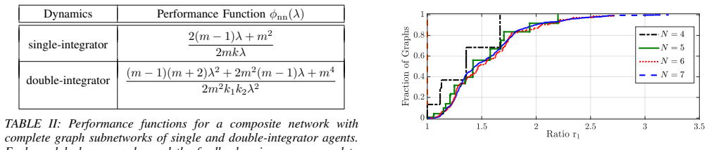
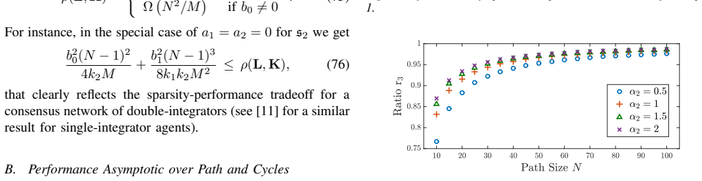
- Over path and cycle graphs, the performance scales as $\Theta(N\Gamma_N)$ with $\Gamma_N$ an explicit integral of $\varphi$, yielding concrete laws such as $\Theta(N^2)$ for single integrators and $\Theta(N^4)$ for double integrators with $C=[1,0]$.
- Non-minimum-phase nodal dynamics impose an unavoidable positive floor $\operatorname{Tr}(E^TP_0E)$ on the achievable performance, independent of graph size or feedback gain.
- The same spectral-sum decomposition also applies to the steady-state variance of the control effort $\rho_u$, giving rational input functions $\varphi_u(\lambda,K)$ that inherit the design and scaling analysis.
Reading between the lines
- Inference: The two-level composite formula (66) could be iterated: building subnetworks of subnetworks would add one spectral sum per level, so a hierarchical network with $d$ levels would have performance expressed as a $d$-fold sum over the Laplacian spectra of the graphs at each level.
- Inference: Because $\varphi$ is rational and low-dimensional, its values can be computed once on a grid of $\lambda$ or fit by regression, as the paper suggests, and then reused to evaluate thousands of candidate topologies; this makes spectral-formula-based topology search a plausible algorithmic route that the paper does not itself develop.
- Inference: The paper's bounds rely on convexity of $\varphi$, yet its aircraft example shows $\varphi_1$ need not be convex; a natural extension is to seek similar lower bounds for non-convex $\varphi$ using monotonicity or majorization constraints on Laplacian spectra, or to characterize exactly which nodal dynamics yield convex $\varphi$.
- Inference: A testable conjecture is that when the identical-subsystem or factored-gain assumptions are mildly violated, the formula should still hold approximately with an error controlled by the deviation from undirected symmetry or by the spread of the nodal matrices; the paper gives no such perturbation bound, so this would be new territory.
Signed reviews
Editorial analysis
A structured set of objections, weighed in public.
Referee Report
Summary. The paper studies a network of N identical linear time-invariant agents coupled by relative output feedback over a weighted undirected graph, with external disturbances and measurement noise. Its main claim (Theorem 1) is that the steady-state variance of the deviation from the network average equals a sum, over the nonzero Laplacian eigenvalues, of a low-dimensional rational function phi(lambda,K) obtained from a decoupled Lyapunov equation. The paper then develops connectivity-threshold design conditions for state-feedback and observer-based output-feedback gains, derives performance lower bounds and scaling laws for path/cycle graphs, extends the framework to composite networks, and illustrates the results with many closed-form examples, including double- and triple-integrator agents, platoons, harmonic oscillators, and an aircraft formation.
Significance. If the central formula is correct after the necessary correction, this is a useful unification and generalization of earlier H2/coherency results for first- and second-order consensus networks to arbitrary identical linear nodal dynamics with output feedback and measurement noise. The main strength of the paper is the explicit separation between the graph spectrum and the low-dimensional gain-dependent rational function, which enables symbolic evaluation, design thresholds, and scaling laws. The paper also provides concrete falsifiable predictions, such as Theta(N^2) and Theta(N^4) scalings for path graphs, and a clean LMI construction for minimum-connectivity gains. The appendices contain detailed derivations, and the numerical examples are broadly consistent with the formulas. The significance is conditional, however, because the printed derivation of the main theorem contains an error in the treatment of the measurement-noise term.
major comments (1)
- [Section IV, Eq. (8), and Proposition 1] The displayed closed-loop equation is not the consequence of the model in Section III. From (2) and (3), y=(I_N tensor H)x + sigma*eta, so u = -(L tensor K)(I_N tensor H)x - sigma(L tensor K)eta, and hence the state equation contains -sigma(L tensor BK)eta, not -(L tensor sigma I_{m3})eta. The printed term is dimensionally inconsistent unless n=m3=q and it omits the factor BK; consequently, a reader who follows (8) literally cannot derive the decoupled system (10), the Lyapunov equation (13), or the sigma-dependent examples. Equation (6) similarly drops the measurement-noise term without comment. The intended model is clear from (10), so this is a mechanical error, but it sits at the base of Theorem 1 and must be corrected, with the dimension relation m3=q stated explicitly and the derivations in Appendix A re-verified against the corrected noise term.
minor comments (8)
- [Section III, Eq. (5)] The centering matrix should act on the performance-output dimension m2, not m1; as printed, z(t) has dimension N*m2, so the first factor should be M_N tensor I_{m2}.
- [Section III, after Eq. (2)] The dimensions q and m3 are never related; because eta_i is added to Hx_i and because the observer formulas use F*gamma_i, the paper should state explicitly that m3=q.
- [Section V.D, Theorem 8, Eq. (37)] The limit in (37) is taken with respect to sigma, but sigma is the physical measurement-noise magnitude fixed by the problem; the dual of Theorem 7 requires an independent auxiliary parameter epsilon, as in (35)-(36), and (38) should be written with epsilon^{-2}. As printed, the statement conflates the design parameter with the noise level.
- [Example 7, Eq. (53)] For C=e1 and sigma=0, Table I gives phi=1/(2 k1 k2 lambda^2), whereas (53) states 1/(k1 k2 lambda^2); if the performance output is the full state, the expression should additionally contain a 1/(2 k2 lambda) term. The displayed formula should be reconciled with Table I.
- [Example 7, Eq. (55)] Compared with Eq. (42), both rational terms appear to be missing a factor 1/lambda^2 in the denominator; as printed, the sigma=0 term is (9 lambda^4 + 11 lambda^3 + 9 lambda^2 + 4 lambda + 1)/(2(3 lambda^2 + 1)), which does not blow up as lambda tends to zero and does not match (42).
- [Appendix E, proof of Theorem 5] Choosing K* = 2*lambda_tilde(K)*K may not stabilize the system because the infimum in (28) need not be attained; the argument should choose some c > lambda_tilde(K) and take K* = c K.
- [Appendix K, proof of Theorem 11] The derivative argument shows that s is nondecreasing rather than strictly increasing unless phi' is strictly increasing; the equality-characterization sentence should be adjusted accordingly.
- [General modeling assumptions] The paper should state explicitly that the exogenous signals are white-noise processes with unit spectral density; the phrase 'Gaussian with unit variance' alone does not imply the H2-norm variance interpretation used in (7).
Circularity Check
No circularity: Theorem 1's spectral sum is derived from the closed-loop model via standard H2/Lyapunov arguments, and no fitted parameter is relabeled as a prediction.
full rationale
The central derivation is self-contained. The paper defines the closed-loop dynamics (2), (3), and (8), then diagonalizes the network through the Laplacian eigenbasis (9) to obtain the decoupled modal systems (10). Proposition 1 and Theorem 1 compute the steady-state variance as the sum of the H2 norms of these modal systems, with P(lambda,K) given as the solution of the Lyapunov equation (13); no free parameter is fitted to the performance data. The rational-function claim follows from Cramer's rule applied to the vectorized Lyapunov equation (Appendix A, Eq. (92)), not from an assumed ansatz. The scaling laws in Theorem 13 and the examples are obtained by inserting known Laplacian eigenvalue formulas for path and cycle graphs into the already-derived phi, and then evaluating or bounding the resulting integral; this is application, not circularity. The only self-citations (e.g., [14] for the conference predecessor, and [1], [2], [11] for prior related work) are historical or comparative and are not load-bearing for the main theorem. The proof does invoke external results — [12] for part of Theorem 5 and [16]/[29] for LMI and graph inequalities — but these are independent published results, not circular self-support. The typographical inconsistency in the displayed noise term of Eq. (8) (dimension mismatch with the intended -lambda_i BK sigma gamma_i term in Eq. (10)) is a correctness or manuscript issue, not a circularity; the derivation chain itself does not reduce to its inputs by construction.
Assumptions & free parameters
free parameters (3)
- feedback gain K
- observer gain F
- connectivity threshold bound c in LMI (30)
assumptions (4)
- domain assumption All subsystems are identical (same A, B, E, H, C) and the feedback gains factor as K_ij = k_ij K over an undirected weighted graph.
- domain assumption Disturbance xi and measurement noise eta are Gaussian, white, uncorrelated, and have unit covariance.
- standard math Stabilizability of (A,B) and detectability of (A,H) are assumed or shown necessary for finite connectivity thresholds.
- standard math Spectral theorem for symmetric Laplacians, Cramer's rule, and standard Lyapunov equation theory.
Cite this review
Pith. "Pith review of Explicit Characterization of Performance of a Class of Networked Linear Control Systems." pith.science (2026). https://pith.science/paper/UB5XLQHC
@misc{pith2026190801421,
  author       = {Pith},
  title        = {Pith review of: Explicit Characterization of Performance of a Class of Networked Linear Control Systems},
  year         = {2026},
  howpublished = {\url{https://pith.science/paper/UB5XLQHC}},
  note         = {Machine review of arXiv:1908.01421}
}
read the original abstract
We show that the steady-state variance as a performance measure for a class of networked linear control systems is expressible as the summation of a rational function over the Laplacian eigenvalues of the network graph. Moreover, we characterize the role of connectivity thresholds for the feedback (and observer) gain design of these networks. We use our framework to derive bounds and scaling laws for the performance of the dynamical network. Our approach generalizes and unifies the previous results on the performance measure of these networks for the case of arbitrary nodal dynamics. We bring extensions of our methodology for the case of decentralized observer-based output feedback as well as a class of composite networks. Numerous examples support our theoretical contributions.
Figures


Figures from the paper (3 more)

Reference graph
Works this paper leans on
-
[12]
On H∞ and H2 performance regions of multi-agent systems,
Z. Li, Z. Duan, and G. Chen, “On H∞ and H2 performance regions of multi-agent systems,” Automatica, vol. 47, no. 4, pp. 797–803, 2011
2011
-
[1]
Network abstraction with guaranteed per- formance bounds,
M. Siami and N. Motee, “Network abstraction with guaranteed per- formance bounds,” IEEE Transactions on Automatic Control , vol. 63, no. 10, pp. 3301–3316, 2018
work page 2018
-
[2]
Growing linear dynamical networks endowed by spectral sys- temic performance measures,
——, “Growing linear dynamical networks endowed by spectral sys- temic performance measures,” IEEE Transactions on Automatic Control, vol. 63, no. 7, pp. 2091–2106, 2017
work page 2017
-
[3]
Scaling laws for consensus protocols subject to noise,
A. Jadbabaie and A. Olshevsky, “Scaling laws for consensus protocols subject to noise,” IEEE Transactions on Automatic Control , vol. 64, no. 4, pp. 1389–1402, 2018
work page 2018
-
[4]
Design of optimal sparse interconnection graphs for synchronization of oscillator networks,
M. Fardad, F. Lin, and M. R. Jovanovi ´c, “Design of optimal sparse interconnection graphs for synchronization of oscillator networks,” IEEE Transactions on Automatic Control, vol. 59, no. 9, pp. 2457–2462, 2014
work page 2014
-
[5]
Per- formance and scalability of voltage controllers in multi-terminal hvdc networks,
M. Andreasson, E. Tegling, H. Sandberg, and K. H. Johansson, “Per- formance and scalability of voltage controllers in multi-terminal hvdc networks,” in 2017 American Control Conference (ACC) . IEEE, 2017, pp. 3029–3034
work page 2017
-
[6]
Coherence in large-scale networks: Dimension-dependent limitations of local feed- back,
B. Bamieh, M. R. Jovanovic, P. Mitra, and S. Patterson, “Coherence in large-scale networks: Dimension-dependent limitations of local feed- back,” IEEE Transactions on Automatic Control , vol. 57, no. 9, pp. 2235–2249, 2012
work page 2012
-
[7]
On the ill-posedness of certain vehicular platoon control problems,
M. R. Jovanovic and B. Bamieh, “On the ill-posedness of certain vehicular platoon control problems,” IEEE Transactions on Automatic Control, vol. 50, no. 9, pp. 1307–1321, 2005
work page 2005
Show all 32 references
-
[8]
String instability in classes of linear time invariant formation control with limited communication range,
R. H. Middleton and J. H. Braslavsky, “String instability in classes of linear time invariant formation control with limited communication range,” IEEE Transactions on Automatic Control , vol. 55, no. 7, pp. 1519–1530, 2010
2010
-
[9]
Stability and robustness of large platoons of vehicles with double-integrator models and nearest neighbor interaction,
H. Hao and P. Barooah, “Stability and robustness of large platoons of vehicles with double-integrator models and nearest neighbor interaction,” International Journal of Robust and Nonlinear Control , vol. 23, no. 18, pp. 2097–2122, 2013
2013
-
[10]
Platooning of connected vehicles with undirected topologies: Robustness analysis and distributed h-infinity controller synthesis,
Y . Zheng, S. E. Li, K. Li, and W. Ren, “Platooning of connected vehicles with undirected topologies: Robustness analysis and distributed h-infinity controller synthesis,” arXiv preprint arXiv:1611.01412 , 2016
2016 arXiv
-
[11]
Fundamental limits and tradeoffs on distur- bance propagation in linear dynamical networks,
M. Siami and N. Motee, “Fundamental limits and tradeoffs on distur- bance propagation in linear dynamical networks,” IEEE Transactions on Automatic Control, vol. 61, no. 12, pp. 4055–4062, 2016
2016
-
[13]
On the smallest eigenvalue of grounded laplacian matrices,
M. Pirani and S. Sundaram, “On the smallest eigenvalue of grounded laplacian matrices,” IEEE Transactions on Automatic Control , vol. 61, no. 2, pp. 509–514, 2015
2015
-
[14]
Spectral performance analysis and design for distributed control of multi-agent systems,
H. K. Mousavi, C. Somarakis, and N. Motee, “Spectral performance analysis and design for distributed control of multi-agent systems,” in 2017 IEEE 56th Annual Conference on Decision and Control (CDC) . IEEE, 2017, pp. 2918–2923
2017
-
[15]
Consensus of linear multi- agent systems with reduced-order observer-based protocols,
Z. Li, X. Liu, P. Lin, and W. Ren, “Consensus of linear multi- agent systems with reduced-order observer-based protocols,” Systems & Control Letters , vol. 60, no. 7, pp. 510–516, 2011
2011
-
[16]
S. Boyd, L. El Ghaoui, E. Feron, and V . Balakrishnan, Linear matrix inequalities in system and control theory . SIAM, 1994
1994
-
[17]
Robust pole placement in lmi regions,
M. Chilali, P. Gahinet, and P. Apkarian, “Robust pole placement in lmi regions,” IEEE transactions on Automatic Control , vol. 44, no. 12, pp. 2257–2270, 1999
1999
-
[18]
Robust non-fragile lq controllers: the static state feedback case,
D. Famularo, P. Dorato, C. T. Abdallah, W. M. Haddad, and A. Jad- babaie, “Robust non-fragile lq controllers: the static state feedback case,” International Journal of control , vol. 73, no. 2, pp. 159–165, 2000
2000
-
[19]
Almost disturbance decoupling with internal stability,
S. Weiland and J. C. Willems, “Almost disturbance decoupling with internal stability,” IEEE Transactions on Automatic Control , vol. 34, no. 3, pp. 277–286, 1989
1989
-
[20]
Leader selection for optimal network coherence,
S. Patterson and B. Bamieh, “Leader selection for optimal network coherence,” inDecision and Control (CDC), 2010 49th IEEE Conference on, 2010, pp. 2692–2697
2010
-
[21]
Gitterman, The noisy oscillator: the first hundred years, from Einstein until now
M. Gitterman, The noisy oscillator: the first hundred years, from Einstein until now. World Scientific, 2005
2005
-
[22]
L/sub 2/disturbance attenuation and performance bounds for linear non-minimum phase square invertible systems,
B. Schwartz, A. Isidori, and T. Tarn, “L/sub 2/disturbance attenuation and performance bounds for linear non-minimum phase square invertible systems,” in Decision and Control, 1996., Proceedings of the 35th IEEE Conference on, vol. 1. IEEE, 1996, pp. 227–228
1996
-
[23]
Estrada index of cycles and paths,
I. Gutman and A. Graovac, “Estrada index of cycles and paths,” Chemical Physics Letters , vol. 436, no. 1, pp. 294–296, 2007
2007
-
[24]
Lecture notes for ee263,
S. Boyd, “Lecture notes for ee263,” Introduction to Linear Dynamical Systems, 2008
2008
-
[25]
Cvx: Matlab software for disciplined convex programming, version 1.21 (2011),
M. Grant and S. Boyd, “Cvx: Matlab software for disciplined convex programming, version 1.21 (2011),” Available: cvxr. com/cvx, 2010
2011
-
[26]
State- space solutions to standard H2 and H∞ control problems,
J. C. Doyle, K. Glover, P. P. Khargonekar, and B. A. Francis, “State- space solutions to standard H2 and H∞ control problems,” IEEE Transactions on Automatic control , vol. 34, no. 8, pp. 831–847, 1989
1989
-
[27]
Lecture notes on lqr/lqg controller design,
J. P. Hespanha, “Lecture notes on lqr/lqg controller design,” Knowledge Creation Diffusion Utilization , 2005
2005
-
[28]
H/sub 2/almost disturbance decoupling problem with internal stability,
A. Saberi, Z. Lin, and A. A. Stoorvogel, “H/sub 2/almost disturbance decoupling problem with internal stability,” in American Control Con- ference, Proceedings of the 1995 , vol. 5. IEEE, 1995, pp. 3414–3418
1995
-
[29]
On sum of powers of the laplacian eigenvalues of graphs,
B. Zhou, “On sum of powers of the laplacian eigenvalues of graphs,” Linear Algebra and its Applications , vol. 429, no. 8-9, pp. 2239–2246, 2008
2008
-
[30]
A lower bound for the laplacian eigenvalues of a graph—proof of a conjecture by guo,
A. E. Brouwer and W. H. Haemers, “A lower bound for the laplacian eigenvalues of a graph—proof of a conjecture by guo,” Linear Algebra and its Applications , vol. 429, no. 8-9, pp. 2131–2135, 2008
2008
-
[31]
Performance limitations of non-minimum phase systems in the servomechanism problem,
L. Qiu and E. J. Davison, “Performance limitations of non-minimum phase systems in the servomechanism problem,” Automatica, vol. 29, no. 2, pp. 337–349, 1993. APPENDIX A Proof of Theorem 1: Let us define m =m1 +m3 The transfer matrix from disturbance and noise [ξT,ηT ]T to cons...
1993
-
[32]
Therefore, N∑ i=2 f(λi)≥s(λN)≥s(1 + ∆), (98) which proves 96
and also [30]). Therefore, N∑ i=2 f(λi)≥s(λN)≥s(1 + ∆), (98) which proves 96. Applying this on a convex φ(λ), (70) is followed. The equality holds if and only if λ2 =··· =λN−1 and λN = 1 + ∆, which happens if and only if G is either complete or star (again, see both [29] and [...
2017
Reviewed August 14, 2026 · model on record in the stance chip above.
Discussion (0). Continue with ORCID to comment.